Figure 1
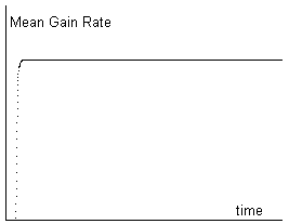
Evolution of Mean Gain Rate with a single adjustment of Supply and Demand
gi = ppi / ki - 1 = gm , and therefore
Abstract
Marx (1894) introduced the concept of "production price" as a result of the full mobility of capital between different sectors of production toward the equalisation of its gain rates. Nevertheless, he doesn't explain this process of equalisation between heterogeneous sectors, and its Law of Decreasing Tendency of the Gain Rate supposes an unjustified equalisation of the plusvalue rates (quotient between the gain and the capital invested in work power).
After, Sweezy (1972) and Salama-Valier (1973) intended to explain the process, but their explanations weren't satisfactory for treating with static situations in equilibrium, when the real evolution is produced from situations of non-equilibrium.
Pla-Lopez (1986) presented a model of System Dynamics of the equalisation of the Gain Rate, which explained the possibility of evolution toward a greater proportion of inversion in production means, and concluded that the Marx's Law of Decreasing Tendency of the Gain Rate was wrong.
Now, we are going to complete the model by introducing the
adaptation
of the Demand to the Incomes, which we name Solvent Demand, and
studying
by computer simulation the results of the model in the evolution of the
Main Gain Rate.
Adjustment of Supply and Demand
We work with classical curves of Supply and Demand (see for example
Lipsey (1967)), with its "elasticity" as exponent. These curves ideally
would determine the Supply and Demand in function of the prices,
Of = kOprEo
Dem = kD
prEd
Of course, usually the elasticity of the Supply will be positive,
Eo>0,
and the elasticity of the Demand will be negative, Ed<0. But the
condition
of equilibrium is that the elasticity of the Demand would be greater in
absolute value than the elasticity of the Supply, |Ed|>|Eo|.
In order to simulate the evolution of the Supply, we suppose that the
Ideal Supply is determined by the real price, and the real Supply Of
tends
lineally toward the Ideal Supply Of with a delay t1,
so that
(1) Ofi = kOi
priEo
(2) Ofi(t+1) = Ofi(t) + (OfIi(t)
- Ofi(t))/t1
for every sector "i". Of course, if the delay t1
is greater, the evolution of the Supply to its Ideal value will be
slower,
and if t1=1 then the Supply equals
its
Ideal value in one step.
Also, in order to simulate the evolution of the Demand to its Ideal
value with equalisation of Supply and Demand, we will suppose that the
Ideal Demand is equal to the real Supply, the Ideal Price is determined
by the Ideal Demand according to the relation (1'), and the real Price
tends lineally toward the Ideal Price with a delay t2,
that is to say
(3) DemIi = Ofi
(4) prIi = (DemIi
/ kDi)1/Ed
(5) pri(t+1) = pri(t)
+ (prIi(t) - pri(t))/t2
(6) Demi = kDipr
Ed
If the condition of equilibrium |Ed|>|Eo| is fulfilled, then this
System
will evolve toward an situation of equilibrium in which
Dem = Dem I
=
Of = Of I = (kDEo
kO-Ed)1/(Eo-Ed)
and
pr = prI = (kD/kO)1/(Eo-Ed).
Equalisation of the Gain Rates
We will suppose that to produce a unity of the product of the sector
"i" we need aij
unities
of the sector "j", so that its unitary cost is
(7) ki = Σj aij
prj
for every sector "i". We consider work power as a sector, so that wages
are included in this unitary cost.
The total cost in a sector "i" will be ki Ofi
,
but its total incomes will be pri mi,
where mi will be the minimum between
its
Supply and its Demand,
(8) mi = min ( Ofi,
Demi )
Therefore, the gain rate in this sector will be gi
= (pri mi
-
ki Ofi)/
ki Ofi =
pri mi /
ki Ofi -
1 .
Because mi ≤ Ofi
, gi ≤
pri / ki -
1 , and therefore, gi > 0 only if
Σj aij
prj< pri
. So, in order to get gi>0 for
every i,
we can take aijso
that ||a||<1, and therefore ||a
pr||<||pr||. We will work with infinite norm, and so we will take aij so
that Σj aij
< 1 (the coefficients aij
are always positive). This condition is not necessary, but if
the
condition
åj
aij
prj
< pri is fulfilled we can
select
the unity of each product in order to get it.
The Mean Gain Rate will be gm = Σi gi
kiOfi /Σj kjOfj , and
therefore
(9) gm = Σi
pri
mi/Σj
kj
Ofj
- 1
If you launch the model with the relations (1) to (5) with the
condition
of equilibrium |Ed|>|Eo| and random coefficients aij so
that Σj aij
< 1 , the Mean Gain Rate increases until reaching the
equilibrium
between Supply of Demand (in fact, out of this equilibrium can
inefficiently
be mi < Ofi
, so that gi < pri/
ki - 1 and gm
< Σi pri
Ofi
/Σj
kjOfj
-1 which is its value in
this equilibrium). We can see an example in the Figure 1.
 Figure 1 Evolution of Mean Gain Rate with a single adjustment of Supply and Demand |
Nevertheless, in this simple equilibrium between Supply and
Demand,
with constant parameters kOi and
kDi , the Gain Rates of
the
different sectors are not equalised. This equalisation requires a
movement
of capital between sectors which will produce a displacement of the
curves
of Supply, through a change of the parameters kOi
,
so that the prices of equilibrium between Supply and Demand will tend
to
the Production Prices ppi in each
sector
"i" so that its Gain Rate were equal to the Main Gain Rate,
gi = ppi / ki - 1 = gm , and therefore |
In order to simulate the evolution of the parameters kOi
,
we will suppose that they tend lineally with a delay t3
to an ideal value kOIi
which corresponds to the Production Price ppi
with the present parameter kDi of
the curve of Demand, so that
(11) kOIi
=
kDi /ppiEo-Ed
(12) kOi (t+1)
= kOi (t) + (kOIi(t)
- kOi (t))/t3
Note that, in conditions of equilibrium, Σj aij ppj = ppi / (1+gm), and therefore 1/(1+gm) has to be a self-value of the matrix aij , and the prices of production form its corresponding self-vector. Therefore, the possible values of Mean Gain Rate in equilibrium, and also the relative proportion of the prices in equilibrium, depend only on the intersectorial coefficients aij (Pla-Lopez 1986).
The relative proportions of the parameters in equilibrium of the
curves
of Supply, kOi , will
also depend
on the parameters of the curves of Demand, kDi.
Of course, according to the relations (11), if the prices in
equilibrium
change in a proportion λ from different initial
conditions, these parameters in equilibrium will change in a proportion
λEd-Eo.
Adjustment to the Solvent Demand
Nevertheless, a Demand is only sustainable if it is Solvent, that is
to say, it can be paid for the corresponding Incomes. In order to study
the adaptation to the Solvent Demand, we will consider only three
sectors:
Sector 0: production of means of production.
Sector 1: production of goods for workers.
Sector 2: production of goods for owners of means of production.
In order to simplify the model, we will suppose that there is a full
division between workers and owners of means of production, and between
sector 1 and sector 2.
In the relations (6), the prices of sector 2 don't contribute to the
unitary cost of any product, and therefore ai2=0
for every sector "i". By the way, the prices of sector 1 contribute to
the unitary cost through the wages (see Sraffa 1960). So, the total
incomes
of the workers (its wages) will be equal to the total cost from the
sector
1, Σi Ofi
ai1
pr1 . Therefore, the Solvent Demand
of
the sector 1 will be DemSi
= Σi
Ofi
ai1
pr1/ pr1
= Σi Ofi
ai1
and according to the relation Dem = kD
prEd its parameter of Solvent
Demand will
be
(13) kSD1
= DemS1/pr1Ed
= Σi Ofi
ai1
/ pr1Ed
and we will suppose that the parameter kD1
tends lineally to this parameter of Solvent Demand with a delay t4
,
(14) kD1(t+1)
= kD1(t) + (kSD1(t)
- kD1(t))/t4
On the other hand, the total incomes of the owners of means of
production
will be its total gain,
Σi pri
mi
- Σi
ki
Ofi. Therefore, the
Solvent
Demand of the sector 2 will be
DemS2 = (Σi
pri
mi- Σi
ki
Ofi
)/ pr2 , and the corresponding
parameter
of Solvent Demand will be
(15) kSD2
= DemS2 / pr2Eo
= (Σi pri
mi
- Σi
ki
Ofi)/ pr2Eo+1
We will also suppose that the parameter kO2
tends lineally to this parameter of Solvent Demand with a delay t4
,
(16) kD2(t+1)
= kD2(t) + (kSD2(t)
- kD2(t))/t4
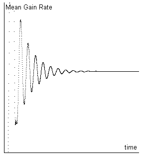
 Figure 2 Evolution of Mean Gain Rate with static technology |
The interaction between the adjustment of Supply and Demand,
the equalisation
of the Gain Rates and the adjustment to the Solvent Demand not always
tends
toward equilibrium. But if so, the Mean Gain Rate oscillates toward its
value of equilibrium, which only depend on the intersectorial
coefficients
which express the technological conditions. In Figure 2 you can see an
example.
On the other hand, in a solvent equilibrium
|
Remember, but, that the unitary cost of a product is ki = ai0 pr0 + ai1 pr1, where ai0 expresses the contribution of the means of production, and ai1 expresses the contribution of the work power through the wages (equal to ai1 pr1). Therefore, these coefficients also express the social relations between workers and owners of means of production, and the unionist struggle can carry to increase the wages, and so it could carry to increase the coefficients ai1. Nevertheless, we can plausibly suppose that the wages increase lesser than the productivity, and so that the coefficients ai1 do not increase, but decrease through technological progress, by means of saving in work power.
The Model uses Ed=-.5 and Eo=.3 (but these values can be easily changed), and demands to fix the values of the delays (we have used t1=t2=t4=10 and t3=t5=20). And, in order to simulate the process without more presuppositions, the Model can fix randomly the initial values of intersectorial coefficients, prices, amount of Supply and parameters of the curves of Supply and Demand. Then, the dynamical relations of the Model can change these values, eventually toward some value of equilibrium of the Mean Gain Rate.

Figure 3
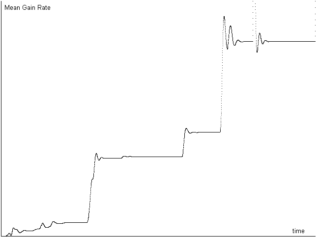
Evolution of Mean Gain Rate through technological
progress
Nevertheless, the technological progress, through a random decreasing of the intersectorial coefficients, can break this equilibrium, and begin an evolution toward a new equilibrium. You can see a typical process in Figure 3: through this technological progress, the Mean Gain Rate increases over its previous value of equilibrium.
You can find the source code of our Model in http://www.uv.es/~pla/models/modpp.c
, and a DOS executable program in http://www.uv.es/~pla/models/modpp.exe
. This is an ANSI C program with only text output, but, of course, you
can adapt the source code to your compiler in order to get a graphical
output, like we have done.
Conclusions and open questions
Through our computer simulation, we have tested and ratified our previous conclusion (Pla-Lopez 1986) about the increasing of the Mean Gain Rate through technological progress. Moreover, its oscillations can explain some economic crisis.
Nevertheless, our Model explores a theoretical situation, without
monopolies
nor ecological bounds of the economic growth. These questions remain
open
to later studies, applications and developments of our Model.
Bibliography
Forrester, J:W. (1968), "Principles of systems", Wright-Allen Press, Cambridge.
Lipsey, R.G. (1967), "Introducción a la economía positiva", Vicens-Vives, Barcelona.
Marx, K. (1894), "El Capital", vol.III, Fondo de Cultura Económica, Mexico, 1959.
Pla-Lopez, R. (1986), "Study by System Dynamics of the Problem of the Equalization of the Gain Rate" in "System Dynamics: on the move", proceedings of the 1986 International Conference of the System Dynamics Society, Sevilla.
Salama, P. and Valier, J. (1973), "Une introduction a l'économie politique", Maspero, Paris.
Sraffa, P. (1960), "Production of Commodities by means of Commodities", Cambridge University Press, Cambridge.
Sweezy, P.M. (1972), "Teoría del desarrollo capitalista",
Fondo
de Cultura Económica, Mexico.