Z-Tests and T-Tests:
One Sample Hypothesis Tests

Gravetter & Wallnau, Chapters 8 & 9
ViSta, Chapter 4

Copyright © 1997-8 by Forrest W. Young.

P30Home Schedule Labs Homework Project Lectures

  1. Overview
  2. Chapter 8 presents the statistical procedures that permit researchers to use a sample mean to test hypotheses about a population. These statistical procedures were based on a few basic notions, which are summarized as follows:

    1. A sample mean is expected to more or less approximate its population mean . This permits us to use the sample mean to test a hypothesis about the population mean.

    2. The standard error provides a measure of how well a sample mean approximates the population mean. The standard error formula is:

    3. To quantify our inferences about the population, we compare the obtained sample mean with the hypothesized population mean by computing a z-score test statistic. The Z-Test statistic's formula is:

    There is one major problem with this:
    We don't usually know the population's standard deviation, which is required to compute the z-score's standard error.

    Chapter 9 presents the statistical procedures that permit researchers to use a sample mean to test hypotheses about a population, when the population standard deviation is NOT known.

    These procedures use the T-Test, rather than the Z-Test. They are based on T-Scores, which we first met in the lecture notes for Topic 4.


  3. The Logic of Hypothesis Testing
  4. We begin by reviewing the logic of hypothesis testing that underlies Z-Tests.

    Example: We return to the example concerning prenatal exposure to alcohol on birth weight in rats. Lets assume that the researcher's sample has n=16 rat pups. We continue to assume that population of normal rats has a mean of 18 grams with a standard deviation of 4.

    Here are the four steps involved in the statistical hypothesis test:

    1. State the Hypotheses:
      • Null hypothesis: No effect for alcohol consumption on birth weight. Their weight will be 18 grams. In symbols:
      • Alternative Hypothesis: Alcohol will effect birth weight. The weight will not be 18 grams. In symbols:
    2. Set the decision criteria:
      • Specify the significance level. We specify:
      • Determine the critical value of Z. We do this for the choosen significance level. For a non-directional test the critical value of Z is the value that has alpha-percent of the area more extreme than Z. For alpha=.05 we look up a Z that has .025 of the distribution beyond it. This is a Z of +1.96 and -1.96.

    3. Gather Data:
      Lets say that two experimenters carry out the experiment, and we get the following two samples of results:
      Experiment 1Experiment 2
      Sample Mean = 13Sample Mean = 16.5

    4. Evaluate Null Hypothesis:
      We calculate the standard error of the mean, then calculate Z for each experiment, and then look up the P value for the obtained Z, and make a decision.
      • Determine the standard error of the mean. The standard error is calculated by the formula:

        The value is 4/sqrt(16) = 1.

      • Calculate the Test-Statistic. To determine how unusual the mean of the sample we will get is, we will use the Z formula to calculate Z for our sample mean under the assumption that the null hypothesis is true. The Z formula is:

        Note that the population mean is 18 under the null hypothesis, and the standard error is 1, as we just calculated. We then can calculate Z by using the obtained sample mean. We then look it up in the Z table to see how unusual the obtained sample's mean is, and decide if the null hypothesis Ho is true.

        Here's what happens for each experiment:

        Experiment 1Experiment 2
        Sample Mean = 13
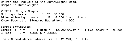
        Z = (13-18)/1 = -5.0
        p < .0000
        Reject Ho
        Sample Mean = 16.5
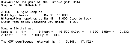
        Z = (16.5-18)/1 = -1.5
        p = .1339
        Do Not Reject Ho

        Here is ViSta's report for these two experiments:

        ViSta Applet
        Report for Univariate Analysis of Experiment 1 Data.

        ViSta Applet
        Report for Univariate Analysis of Experiment 2 Data.


  5. T --- A Substitute for Z
  6. The limitation of Z-Tests is that we don't usually know the population standard deviation. What we do is:
    When we don't know the population's variability, we assume that the sample's variability is a good basis for estimating the population's variability.
    Recall, from
    Chapter 4, that the sample variance and sample standard deviation are unbiased estimates of the population variance and populatin standard deviation.

    The formula for the sample variance is:

    The formula for the sample standard deviation is:

    Using these sample values, we can estimate the standard error of the distribution of sample means. As stated above (and developed in Chapter 8), the formula for the standard error is:

    The estimate of the standard error is simply:

    We use the estimate of the standard error to define the T-statistic:

    Note the parallelism between Z and T
    Known Population Variance Unknown Population Variance

    T-Statistic
    The T-Statistic is used to test hypotheses about the population mean when the value for the population variance is unknown. The formula for the T-Statistic is similar in structure to that for the Z-Statistic, except that the T-Statistic uses estimated standard error rather than the (unknown) standard error.

  7. Using T
  8. The process of hypothesis testing when we don't know the population standard deviation is the same as the process when we do know it.

    We have the same four steps. The only differences are in determining the critical region and in calculating the standard error.

    1. State the Hypotheses:
      This step is the same as with the Z-Statistic.

    2. Set the decision criteria:
      • Specify the significance level.
        This is the same as with the Z-Statistic.
      • Determine the critical value of T.
        Here there is a new complication in using T: There isn't just one T-distribution that we use to determine the critical value of T. There is a whole family of distributions. The distribution depends on the "degrees of freedom", which is simply equal to one less than the sample size. That is:

        We locate the critical T value by using the T distribution table in the Appendix.

    3. Gather Data.
      This step is the same as with the Z-Statistic.

    4. Evaluate the Null Hypothesis.
      We calculate the standard error of the mean using the sample's standard deviation. Then we calculate T and look up the P value for the obtained T and known df. Then we make a decision.
      • Determine the standard error of the mean. The standard error is calculated by the formula:

      • Calculate the Test-Statistic. The T formula is:
    Example: Eyespot Data

    Many accounts suggest that many species of animals find direct stares from another animal aversive. Some moths have developed eye-spot patterns on their wings or bodys to ward off predators. An experiment was done using 16 moth-eating birds. These birds were tested in a two-chambered box that they were free to roam in from side to side. One chamber had two eye-spot patterns painted on the wall. The other chamber had plain walls. Each bird was left in the chamber for 60 minutes, and the amount of time spent in the plain chamber was recorded.

    Here are the four steps involved in the statistical hypothesis test:

    1. State the Hypotheses: The null hypothesis is that there is no effect for eye-spots painted on the wall. Birds should spend half their time -- 30 minutes -- in each room. The alternative hypothesis is that there is an effect. In symbols the null and alternative hypotheses are:
    2. Set the decision criteria: We arbitrarily decide on an alpha level

      We also note that there are 15 degrees of freedom:

      The table tells us that the critical region consists of t values less than -2.131 and greater than +2.131.

    3. Gather Data:
      Results:

      The mean is 35 minutes in the plain side, and the sample variance is 81.

    4. Evaluate Null Hypothesis:
      Calculations:
      The formula for the estimated standard error is:

      For these data, the estimated standard error is Sqrt(81/16) = 2.25

      The formulat for T is:

      Thus, for these data, T = (35-30)/2.25 = 2.22

      Decision:
      Since 2.22 is in the critical region, we reject the null hypothesis that the presence of eye-spot patterns does not influence behavior.

      ViSta Applet
      Report for the Eyespots Data.


    5. Two more ViSta examples
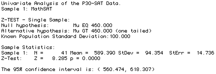
      1. Z-Test: In-class survey SAT Math and Verbal data (pop mean=460, pop stdv=100). ViSta Data

        Report for the SAT Verbal Variable
        Report for the SAT Math Variable

      2. T-Test: Newcomb Lightspeed ViSta Data

        These data are from the first experiment to determine the speed of light. The best modern measurements correspond to a passage time of 33.02 in this experiment. The population standard deviation is unknown.

        Report for the Newcomb Lightspeed Data