Measurements of Numerical Viscosity and Resistivity in Eulerian MHD codes
CAMAP group - Miguel Ángel Aloy - University of Valencia
November 2016
This web page is meant to provide a quick and easy access to the data of the paper:
ON THE MEASUREMENTS OF NUMERICAL VISCOSITY AND RESISTIVITIY IN EULERIAN MHD CODES,
Tomasz Rembiasz, Martin Obergaulinger, Pablo Cerdá-Durán, Miguel-Ángel Aloy and Ewald Müller,
ApJS submitted (2016).
The purpose is to provide the community with actual data to compare with and to serve as a repository for comparison of different Eulerian MHD codes.
The figures in this page are numbered as in the text of the aforementioned paper, which can be found here arXiv.
Below you can find the data with which each figure is produced in ASCII format and the corresponding figure. Note that for each case one needs to perform different transformations on the data, which we explain also below. Should you have more questions or further requests, please, do not hesitate to contact us.
Damping of sound waves
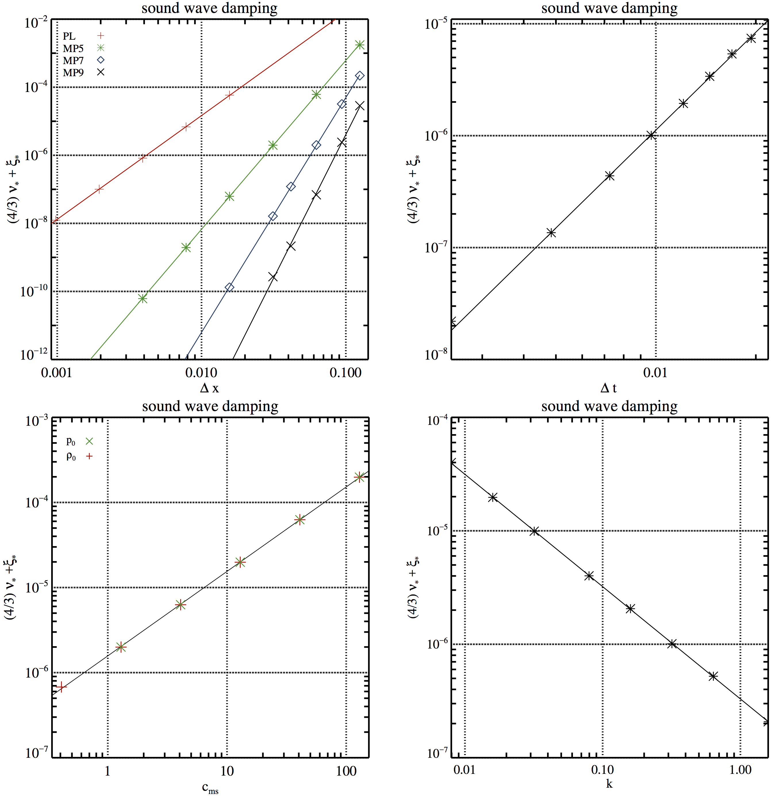
Figure 1. Numerical dissipation of sound waves. Upper left panel: dependence on the grid resolution ∆x for different reconstruction schemes (PL/#S1, MP5/#S3, MP7/#S5, and MP9/#S6), the RK4 time integrator, and \(C_{CFL} = 0.01\). Upper right panel: dependence on the size of the time step size ∆t (by varying \(C_{CFL}\)) for a grid of 64 zones and the MP9 reconstruction scheme (#S8). Lower left panel: dependence on the sound speed for two simulations series in which we kept the background density \(\rho_0\) constant but varied the background pressure \(p_0\) (#cS1, green crosses), and in which we kept \(p_0\) constant but varied \(\rho_0\) (#cS2, red plus signs). Lower right panel: dependence on the wavenumber k = 2π/λ, i.e. on the box size (#cS3). The results shown in the two lower panels were obtained using 32 zones, the MP5 scheme, the RK3 time integrator, and \(C_{CFL} = 0.01\). Straight lines are fits to the simulation results.
Data files for Figure 1.
In the following files \(\Delta x= L / N_x\), where \(N_x\) is the number of points in the \(x-\)direction and \(L = 1\) is the domain length. The following ASCII files correspond to the measured data for each of the cases represented in every panel of the Fig. 1. The data is provided in two-column format, where the first column is \(N_x\) and the second column is minus the damping rate for sound waves \(-\mathfrak{D}_s\).
Left upper panel data PL, MP5, MP7, MP9.
Right upper panel data. The following files include the \(C_{CFL}\) factor (first column), and minus the damping rate for magnetosonic waves, \(-\mathfrak{D}_{s}\). The different tests are set such that the time step is \(\Delta t = C_{CFL} \Delta x / c_{ms}\), computed for a fixed resolution \(\Delta x = 1/64\) and \(c_{ms}=1\). Panel data.
Left lower panel data \(p_0\), \(\rho_0\).
Damping of Alfvén waves
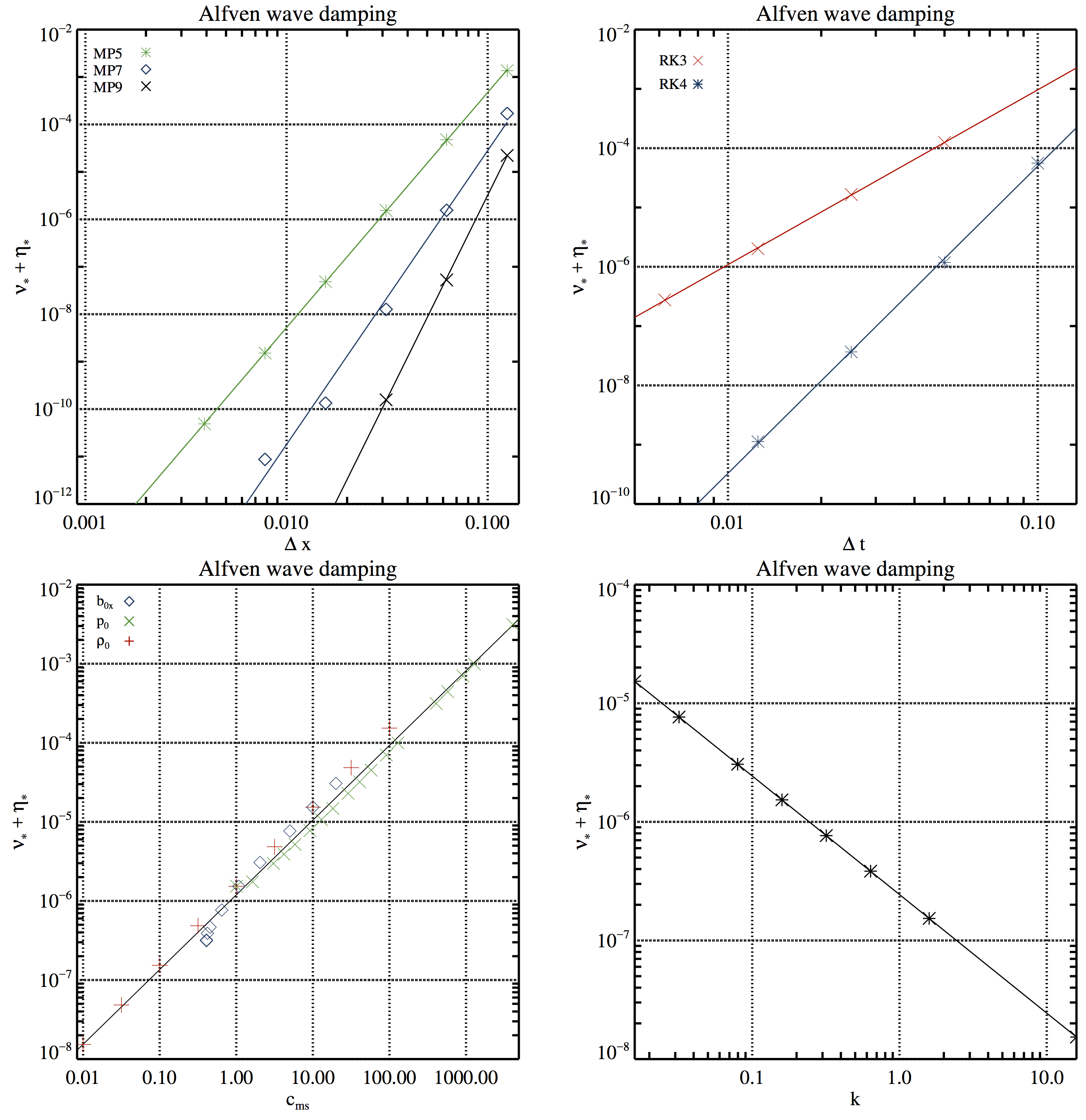
Figure 2. Numerical dissipation of Alfvén waves. Upper left panel: dependence on the grid resolution ∆x for three different reconstruction schemes (MP5/#A2, MP7/#A3, and MP9/#A4) using RK4 and \(C_{CFL} = 0.01\). Upper right panel: dependence on the time step size ∆t (changing the grid resolution but keeping \(C_{CFL} = 0.8\)) for two different time integrators (#A6, and #A7) using the HLL Riemann solver and MP9. Lower left panel: dependence on the fast magnetosonic speed for three simulation series varying the background magnetic field strength b0x (#cA1, blue diamonds), the background pressure \(p_0\) (#cA2, green crosses), and the background density \(\rho_0\) (#cA3, red plus signs) keeping all other parameters constant. Lower right panel: dependence on the wavenumber k = 2π/λ, i.e. on the box size #cA4. Straight lines are fits to the simulation results.
Data files for Figure 2.
In the following files \(\Delta x= L / N_x\), where \(N_x\) is the number of points in the \(x-\)direction and \(L = 1\) is the domain length. The following ASCII files correspond to the measured data for each of the cases represented in every panel of the Fig. 2.
Left upper panel data MP5, MP7, MP9.
Right upper panel data. The following files include the \(C_{CFL}\) factor (first column), and minus the damping rate for magnetosonic waves, \(-\mathfrak{D}_{A}\). The different tests are set such that the time step is \(\Delta t = C_{CFL} \Delta x / c_{ms}\), computed for a fixed resolution \(\Delta x = 1/64\) and \(c_ms=1\). RK3, RK4.
Left lower panel data \(b_x\), \(p_0\), \(\rho_0\).
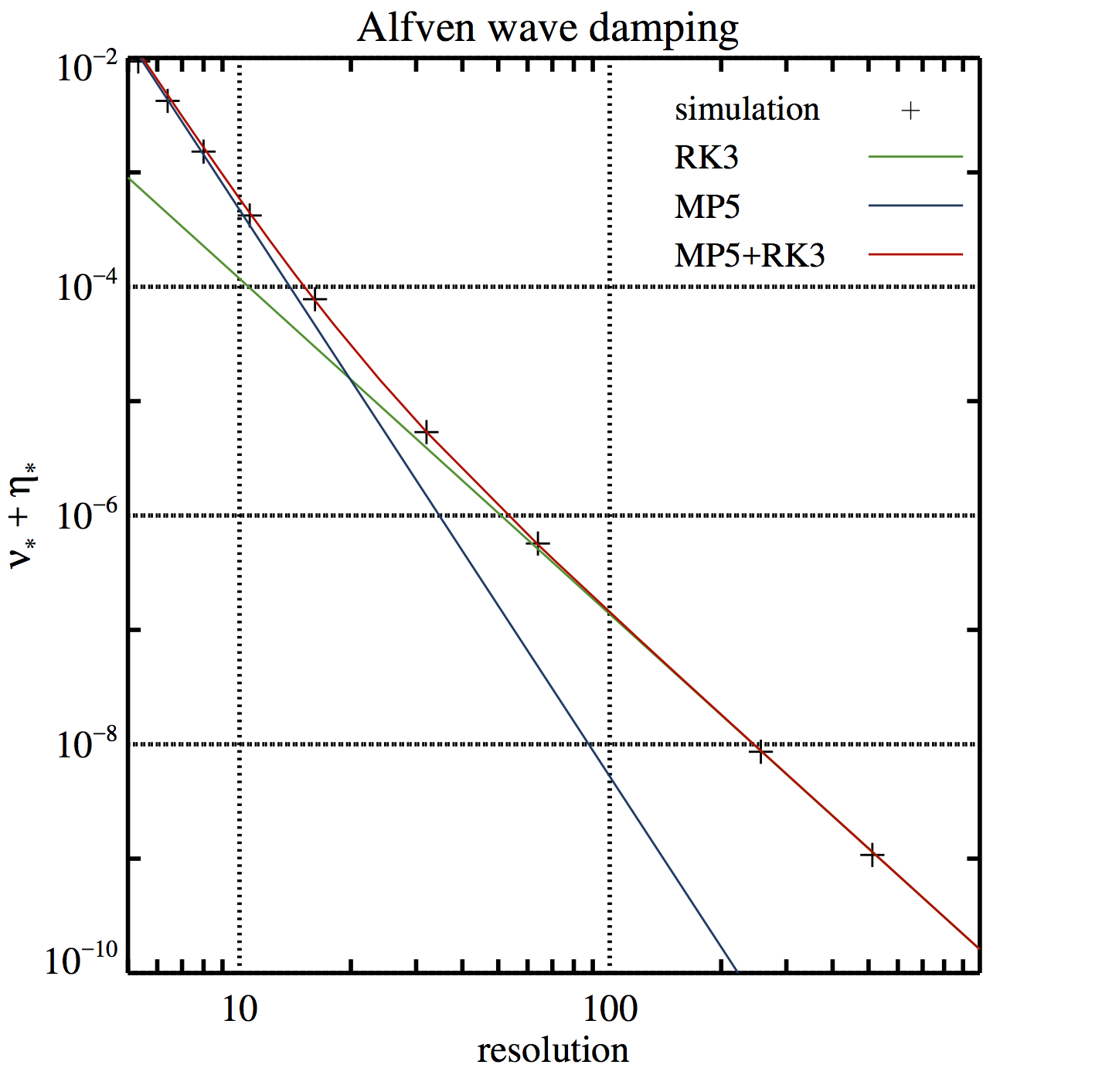
Figure 3. Numerical dissipation as a function of grid resolution for the MP5 reconstruction scheme and the RK3 time integrator with \(C_{CFL} = 0.5\). The simulation results are marked with black plus signs. The straight lines depict the predicted numerical dissipation of the RK3 time integrator (green), the MP5 scheme (blue), and the sum of both types of numerical dissipation (red). For a grid resolution ≤ 16 zones, Alfvén waves are mainly damped by spatial discretisation errors, and for ≥ 128 zones by time integration errors. In the intermediate regime (16, …, 128 zones), both types of errors add linearly (like proper scalars).
Damping of Magnetosonic waves
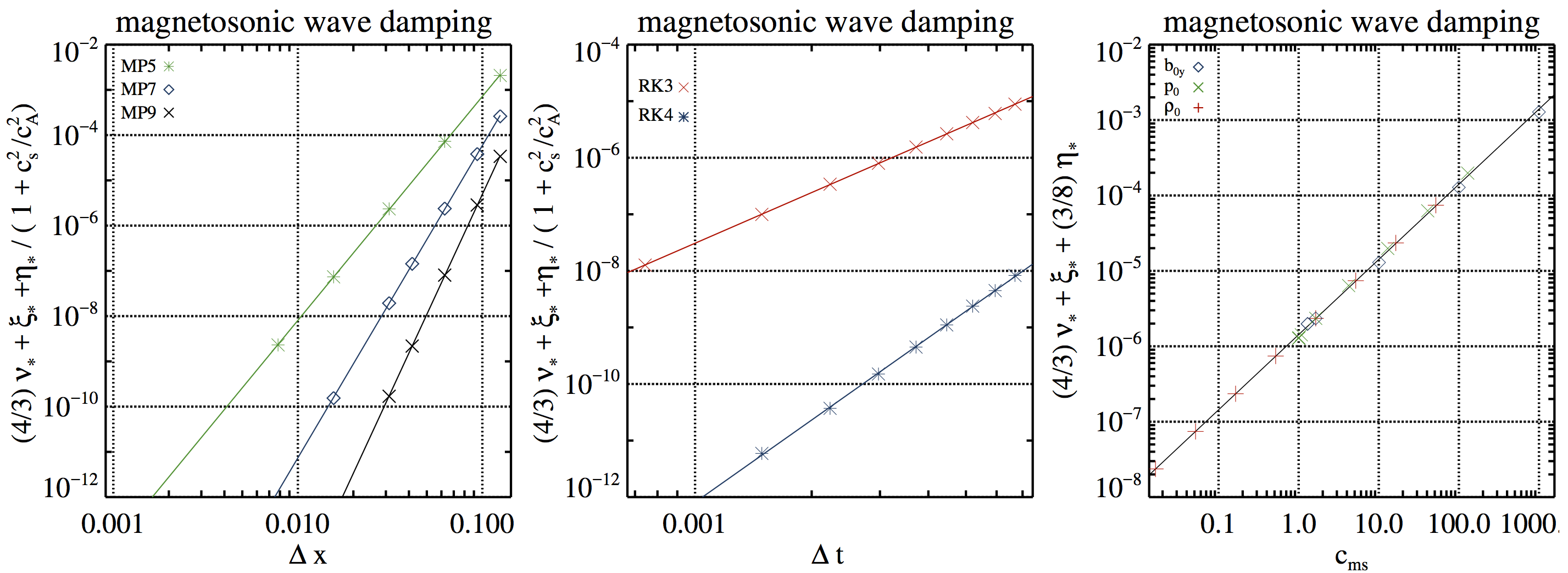
Figure 4. Numerical dissipation of magnetosonic waves. Left panel: dependence on the grid resolution ∆x for three different reconstruction schemes (MP5/#MS1, MP7/#MS2, and MP9/#MS3) using a HLL Riemann solver, RK4, and \(C_{CFL} = 0.01\). Middle panel: dependence on the time step size ∆t for two different time integrators (RK3/#MS4 and RK4/#MS5) using the HLL Riemann solver, MP9, and a grid resolution of 64 zones. Right panel: dependence on the fast magnetosonic speed for simulations varying the background magnetic field strength \(b_{0y}\) (#cMS1, blue diamonds), the background pressure \(p_0\) (#cMS2, green crosses), and the background density \(\rho_0\) (#cMS3, red plus signs) keeping all other parameters constant. Straight lines of are fits to the simulation results.
Data files for Figure 4.
The following ASCII files correspond to the measured data for each of the cases represented in every panel of the Fig. 4.
Left panel data. In the following files \(\Delta x= L / N_x\), where \(N_x\) is the number of points in the \(x-\)direction and \(L = 1\) is the domain length. MP5, MP7, MP9.
Central panel data. The following files include the \(C_{CFL}\) factor (first column), and minus the damping rate for magnetosonic waves, \(-\mathfrak{D}_{ms}\). The different tests are set such that the time step is \(\Delta t = C_{CFL} \Delta x / c_{ms}\), computed for a fixed resolution \(\Delta x = 1/64\) and \(c_{ms}=1\). RK3, RK4.
Right panel data \(b_{0y}\), \(p_0\), \(\rho_0\).
Tearing modes
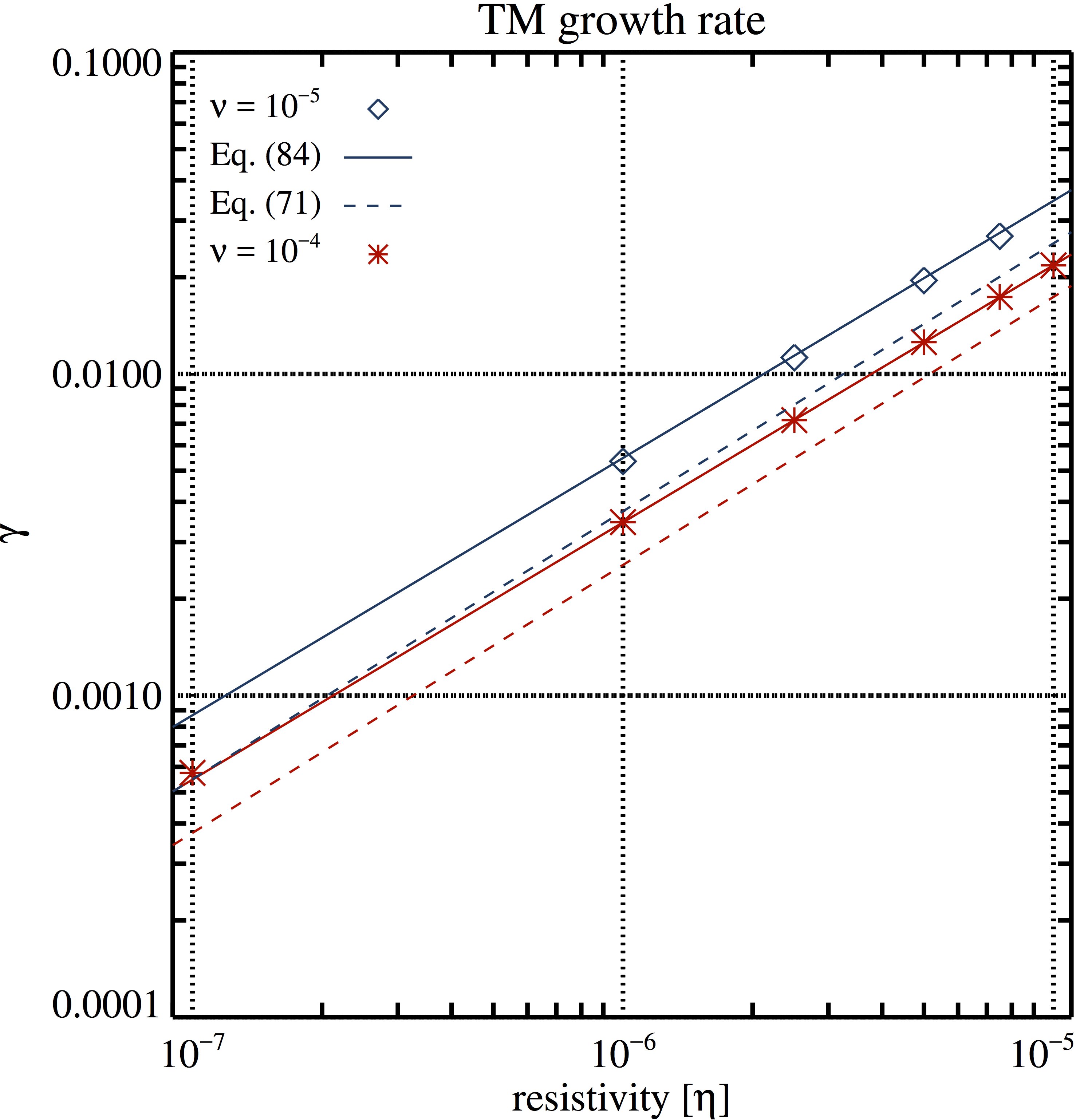
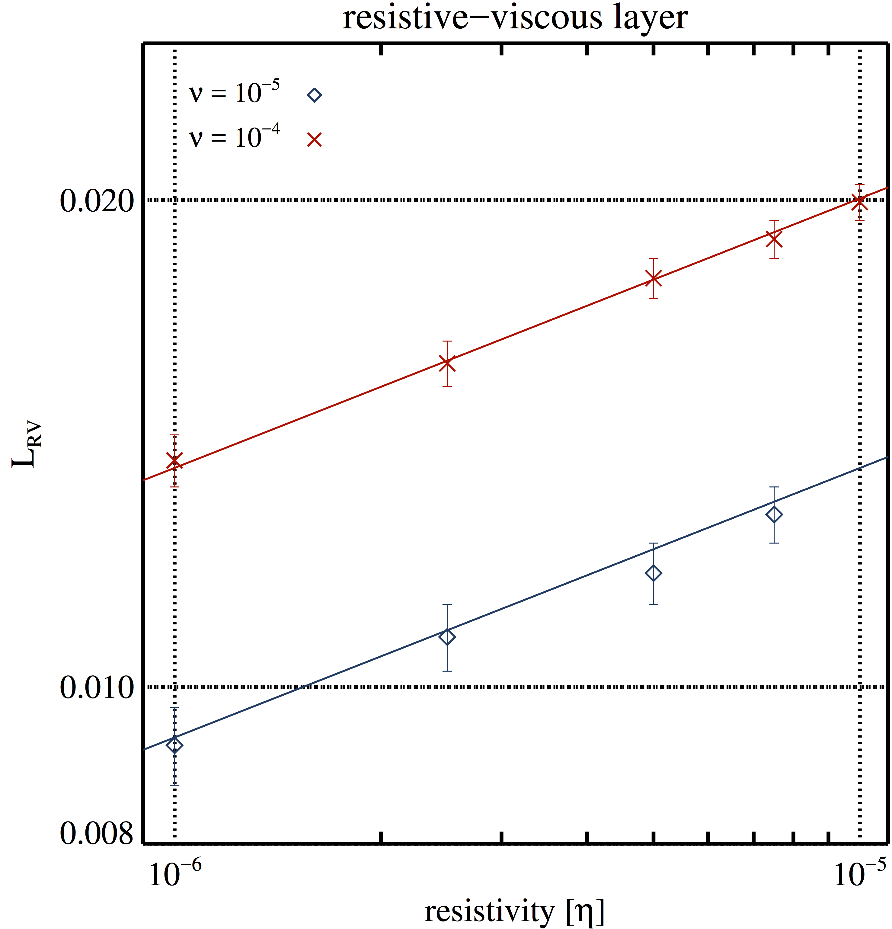
Figure 10. TM growth rate (left) and resistive-viscous layer width (right) as a function of resistivity. Blue diamonds and red asterisks denote results of simulations performed with a constant viscosity of \(\nu = 10^{−5}\) and \(\nu = 10^{−4}\), respectively. The simulations employed the HLL Riemann solver, MP9, and a grid resolution of 2048 × 2048 zones. The solid lines are empirical expressions given by \[\gamma(k=3,a = 0.1)=34.56 \eta^{4/5} \nu^{-1/5} \left(\frac{b_0}{\sqrt{\rho_0}} \right)^{2/5}\] and \[L_{\mathrm{RV}} (k=3,a=0.1)=0.634 (\eta \nu)^{1/6} \left(\frac{b_0}{\sqrt{\rho_0}} \right)^{-1/3},\] respectively. The dashed lines in the left panel are the analytically predictions given by \[\gamma \approx 0.84 \eta^{5/6} \nu^{-1/6} \left( \frac{b_0 k}{\sqrt{\rho_0}}\right)^{1/3} a^{-4/3} \left( \frac{1}{ a\, k }- a\, k \right).\]
Data files for Figure 10.
The following ASCII files correspond to the measured data for each of the cases represented in every panel of the Fig. 10.
Left panel data \(\nu = 10^{−5}\), \(\nu = 10^{−4}\),
Right panel data \(\nu = 10^{−5}\), \(\nu = 10^{−4}\).
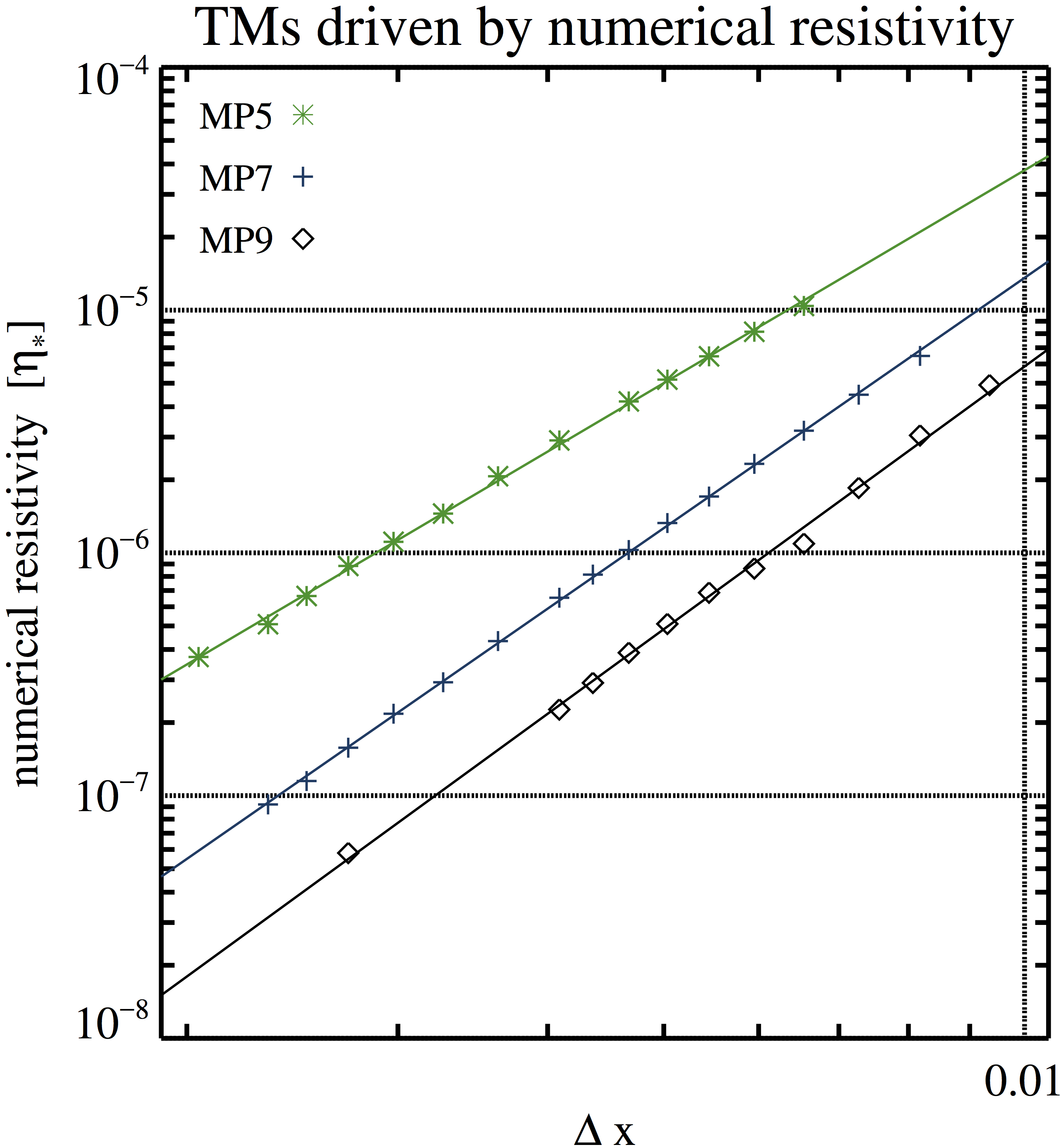

Figure 11. Numerical resistivity of TM simulations performed with 224 to 1024 zones (per dimension), the LF Riemann solver, a viscosity \(\nu = 10^{−4}\), no (physical) resistivity, and the MP5 (green asterisks), MP7 (blue plus signs), and MP9 reconstruction scheme (black diamonds). The straight lines are linear fits to the data.
Data files for Figure 11.
The following files are organized as follows. First column: \(\Delta x = L/N_x\), where \(L=2\pi/3\); Second column: growth rate. To calculate the numerical resistivity we employ \[\eta_{\ast} = \left( \frac{ \gamma(k=3,a = 0.1) }{34.56} \right)^{5/4}\nu^{1/4} \left( \frac{\sqrt{\rho_0}}{b_0} \right)^{1/2}.\] MP5, MP7, MP9.
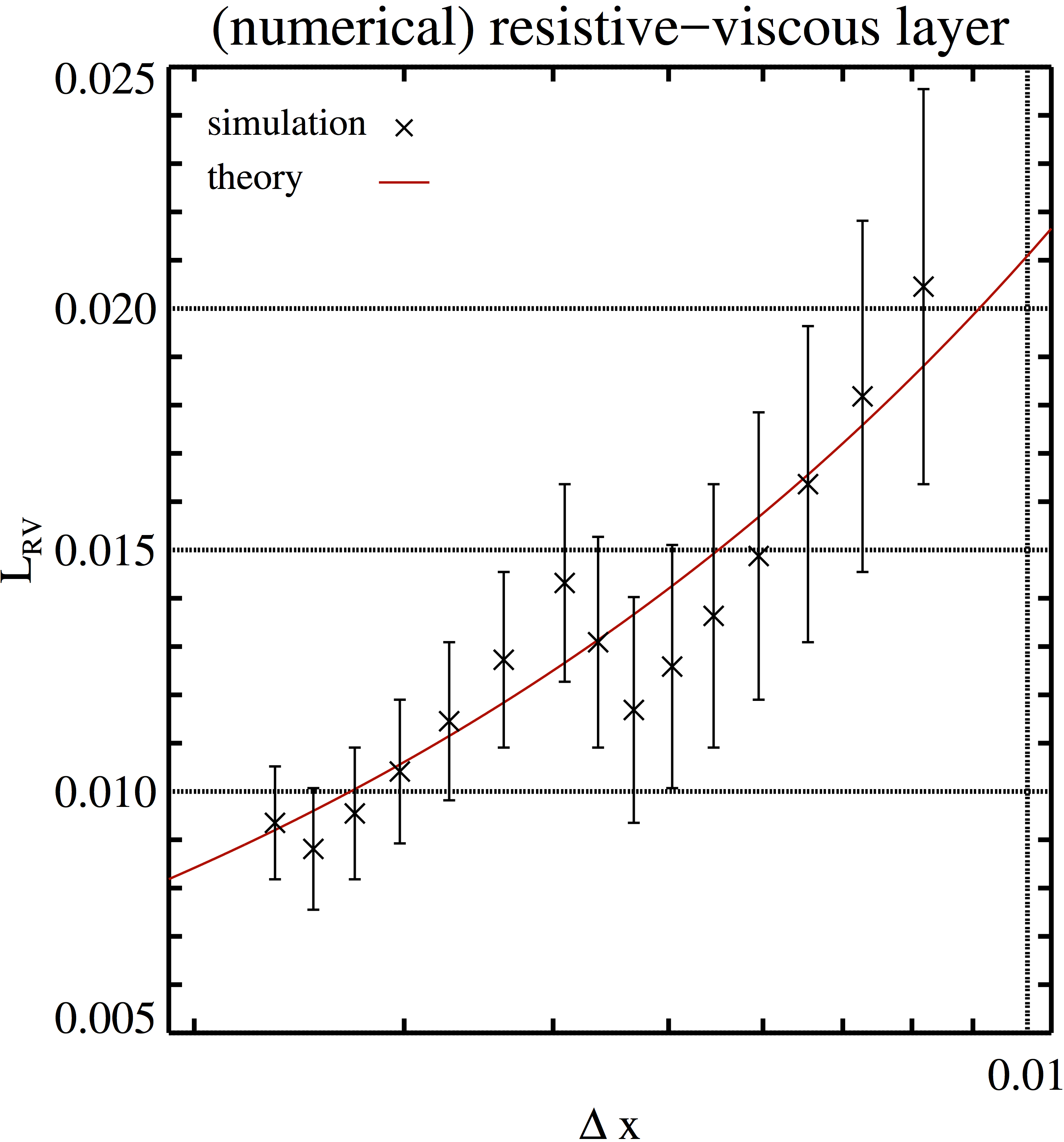
Figure 12. Width of the resistive-viscous layer as a function of ∆x (which is proportional to the value of the numerical resistivity) in simulations of TM driven by numerical resistivity. Black crosses depict measured values obtained in simulations with MP7. The red curve shows the expected layer width \[L_{{\mathrm{RV}}}=\left [ \frac{0.2596}{4^r} \nu \left(\frac{b_0}{\sqrt{\rho_0}}\right)^{-2}\mathfrak{N}_{\eta}^{\Delta x} \mathcal{V} (\Delta x)^{ r} \right ]^{1/(5+r)},\]
given the parameters for the numerical resistivity determined from the measured growth rate.
Data files for Figure 12.
Simulation data. The file is organized as follows.
First column: \(\Delta x = 2\pi/(3N_x)\).
Second column: width of the resistive viscous layer \(L_{RV}\).
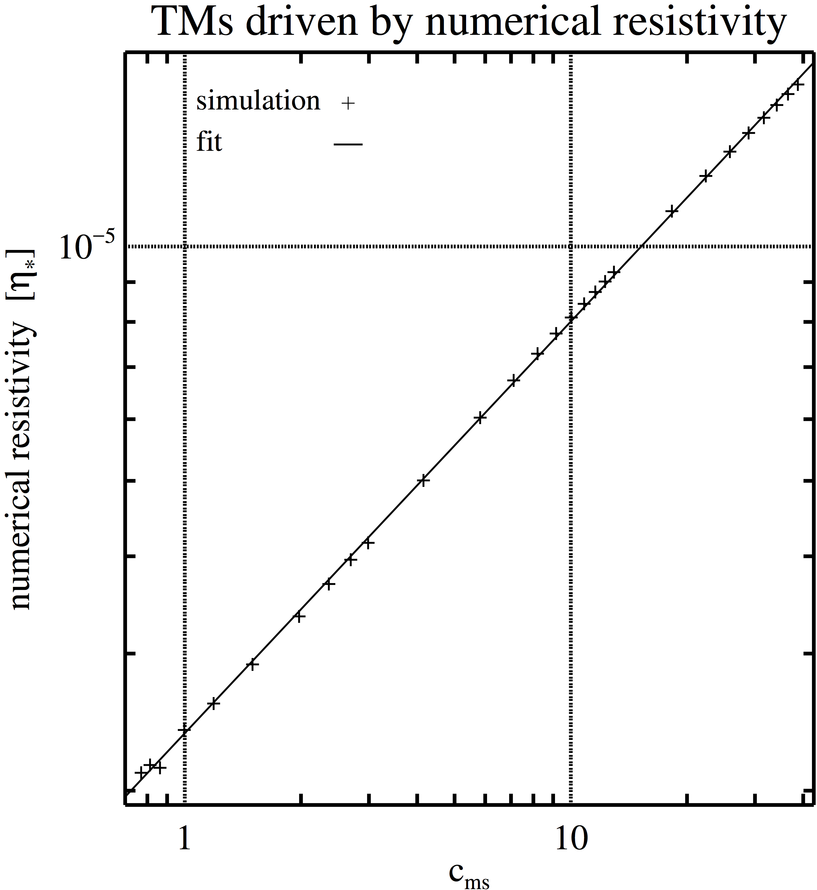
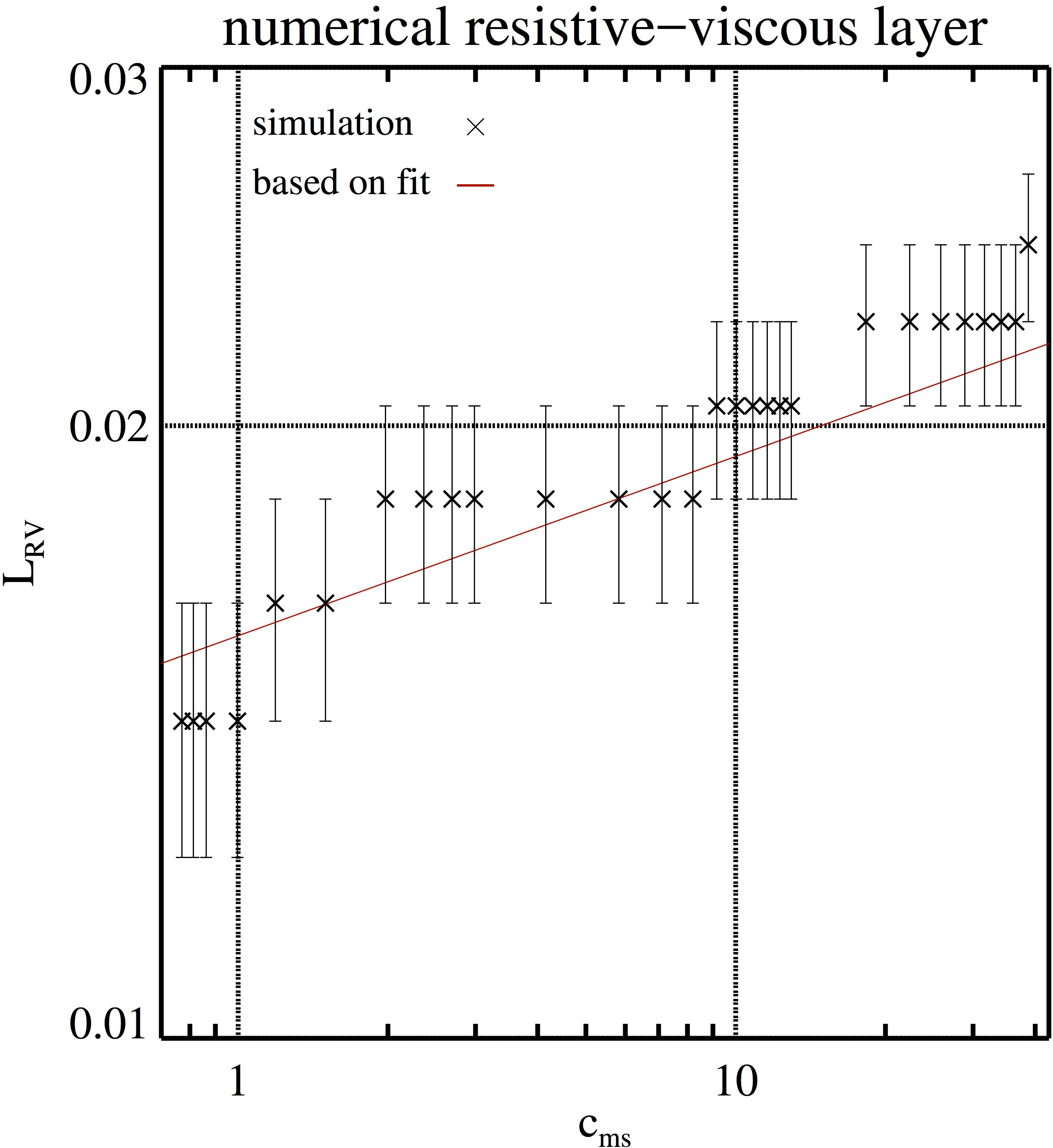
Figure 13. Left panel: Numerical resistivity in TM simulations performed with MP5 on a grid of 512 × 512 zones as a function of the fast magnetosonic speed, \(c_{ms}\), \[c_{\mathrm{ms}} = \sqrt{ 5/3 p_0 + 0.76^2 },\] in this case, which was changed varying \(p_0\) but keeping \(b_0\) and \(\rho_0\) constant. The black curve is a fit to the simulation data. Right panel: Width of the resistive-viscous shear layer (black crosses) as a function of \(c_{ms}\) for the simulations shown in the upper panel. The red curve gives the predicted width of the resistive-viscous layer based on the fit in the upper panel.
Data files for Figure 13.
Left Panel: The data file is organized as follows.
First column: \(p_0\). Second column: growth rate.
To calculate the numerical resistivity we employ \[ \eta_{\ast} = \left( \frac{ \gamma(k=3,a = 0.1) }{34.56} \right)^{5/4} \nu^{1/4} \left( \frac{\sqrt{\rho_0}}{b_0} \right)^{1/2}.\]
Right Panel: Simulation data.
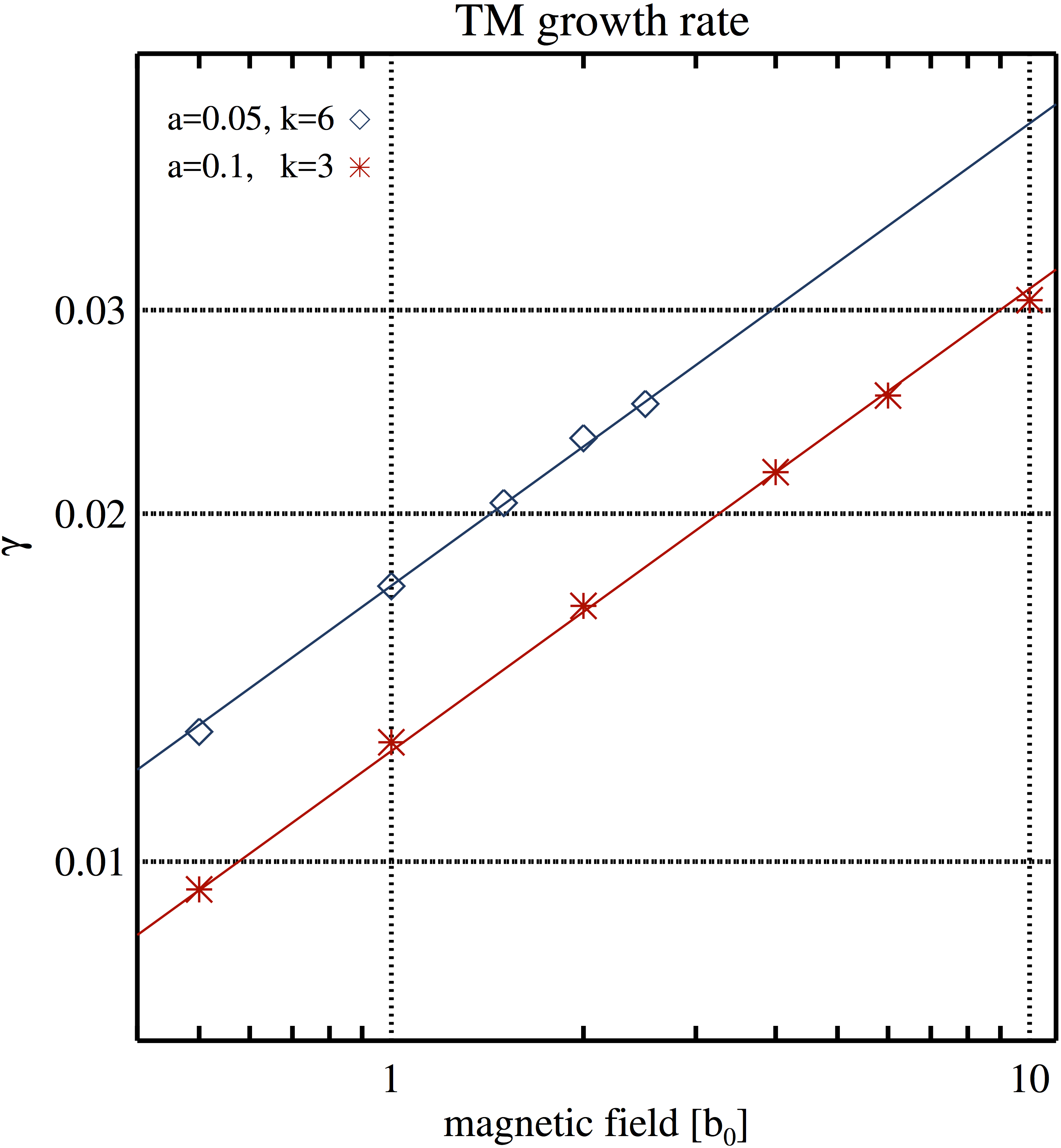
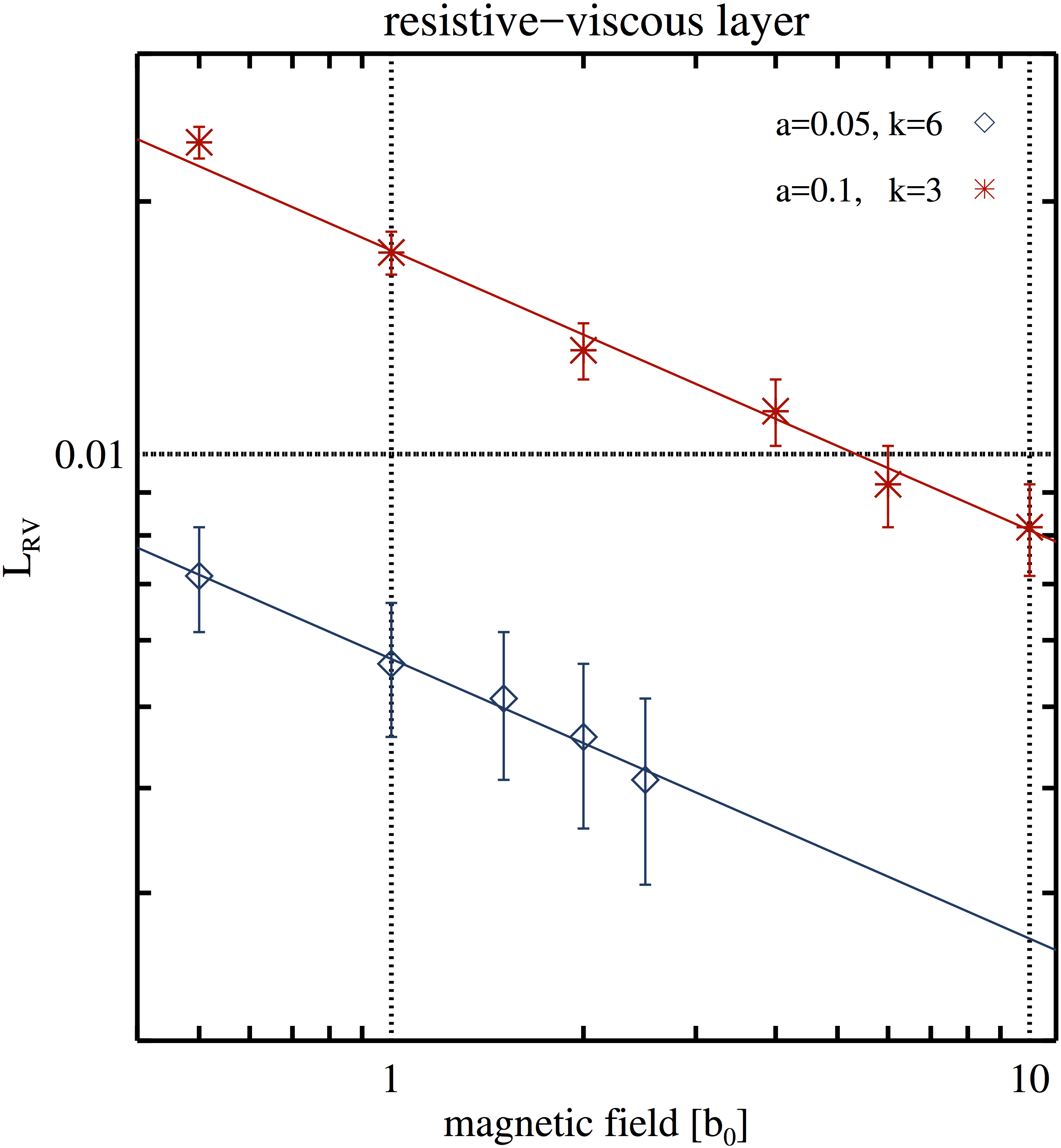
Figure A2. TM growth rate (left) and resistive-viscous layer width (right) as a function of background magnetic field strength. Simulations #TMd and #TMc are depicted with blue diamonds and red asterisks, respectively. Straight lines of the corresponding colours are linear fits to the logarithms of the simulation data.
Data files for Figure A2.
Left Panel: a=0.05, k=6, a=0.10, k=3.
Right Panel: a=0.05, k=6, a=0.10, k=3.