- Definition of Analysis of Variance
- Analysis of Variance (ANOVA) is a hypothesis testing procedure that is used to evaluate differences between the means of two or more treatments or groups (populations). ANOVA uses sample data to make inferences about populations.
- Goals of ANOVA
- Conceptually, the goal of ANOVA is to determine the amount of variability in groups of data, and to see if the variability is greater between groups than within groups.
- ANOVA & T-Tests:
- ANOVA is a more general version of the t-test in two ways:
- Both tests use sample data to test hypotheses about population means. ANOVA, however, can test hypotheses about two or more population means. The T-Test can only test hypotheses about two population means.
- T-Test can only be used with one independent (classification) variable, whereas ANOVA can be used with more any number of independent (classification) variables.
Like the T-Test, ANOVA can be used with either independent or dependent measures designs. That is, the several measures can come from several different samples (independent measures design), or they can come from repeated measures taken on the same sample of subjects (repeated --- dependent --- measures design).
Coverage
- Chapter 13 covers only the very simplest type of ANOVA: One-Way Independent Measures ANOVA (called "single-factor Independent Measures" designs in the book).
- Chapter 14 covers one-way (single-factor) repeated measures designs. We don't cover this.
- Chapter 15 covers two-way independent measures designs. I'll talk about this briefly.
- Example:
- This is hypothetical data from an experiment examining learning performance under three temperature conditions. There are three separate samples, with n=5 in each sample. These samples are from three different populations of learning under the three different temperatures. The dependent variable is the number of problems solved correctly.
Independent Variable:
Temperature (Farenheit)Treatment 1
50-FTreatment 2
70-FTreatment 3
90-F0
1
3
1
04
3
6
3
41
2
2
0
0Mean=1 Mean=4 Mean=1 This is a one-way, independent-measures design. It is called "one-way" ("single-factor") because "Temperature" is the only one independent (classification) variable. It is called "independent-measures" because the measures that form the data (the observed values on the number of problems solved correctly) are all independent of each other --- they are obtained from seperate subjects.
- Hypotheses:
- In ANOVA we wish to determine whether the classification (independent) variable affects what we observe on the response (dependent) variable. In the example, we wish to determine whether Temperature affects Learning.
In statistical terms, we want to decide between two hypotheses: the null hypothesis (Ho), which says there is no effect, and the alternative hypothesis (H1) which says that there is an effect.
In symbols:
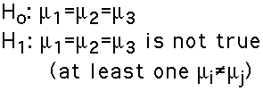
Note that this is a non-directional test. There is no equivalent to the directional (one-tailed) T-Test. - The t test statistic for two-groups:
- Recall the generic formula for the T-Test:

For two groups the sample statistic is the difference between the two sample means, and in the two-tail test the population parameter is zero. So, the generic formula for the two-group, two-tailed t-test can be stated as:

(We usually refer to the estimated standard error as, simply, the standard error). - The F test statistic for ANOVA:
- The F test statistic is used for ANOVA. It is very similar to the two-group, two-tailed T-test. The F-ratio has the following structure:

Note that the F-ratio is based on variance rather than difference.But variance is difference: It is the average of the differences of a set of values from their mean.
The F-ratio uses variance because ANOVA can have many samples of data, not just two as in T-Tests. Using the variance lets us look at the differences that exist between all of the many samples.
- The numerator : The numerator (top) of the F-ratio uses the variance between the sample means. If the sample means are all clustered close to each other (small differences), then their variance will be small. If they are spread out over a wider range (bigger differences) their variance will be larger. So the variance of the sample means measures the differences between the sample means.
- The denominator : The denominator (bottom) of the F-ratio uses the error variance, which is the estimate of the variance expected by chance. The error variance is just the square of the standard error. Thus, rather than using the standard deviation of the error, we use the variance of the error. We do this so that the denominator is in the same units as the numerator.
| Independent Variable: Temperature (Farenheit) |
||
|---|---|---|
| Treatment 1 50-F |
Treatment 2 70-F |
Treatment 3 90-F |
| 0 1 3 1 0 |
4 3 6 3 4 |
1 2 2 0 0 |
| Mean=1 | Mean=4 | Mean=1 |
The most obvious thing about the data is that they are not all the same: The scores are different; they are variable.
- The goals of ANOVA:
- To measure the amount of variability;
- To explain where it comes from.
- Total Variability:
- Our measure of the amount of variability is simply the variability of all of the data: We combine all of the data in the experiment together and calculate its variability.
-
Once we have defined our measure of the total amount of variability, we wish to explain where it comes from: Does it come from the experimental treatment, or is it just random variation? We answer this question by analyzing the sources of variability:
- Between-Treatments Variability:
- Looking at the data above, we can clearly see that much of the variability is due to the experimental treatments: The scores in the 70-F condition tend to be much higher than those in the other conditions: The mean for 70-F is higher than for 50-F and 90-F. Thus, we can calculate the variability of the means to measure the variability between treatments.
- Mean Square Between: The between-treatments variability is measured by the variance of the means. In ANOVA it is called the mean square between. For these data:

- Mean Square Between: The between-treatments variability is measured by the variance of the means. In ANOVA it is called the mean square between. For these data:
- Within-Treatment Variability:
- In addition to the between-treatments variability, there is variability within each treatment. The within treatments variability will provide a measure of the variability inside each treatment condition.
- Mean Square Within: The within-treatment variability measure is a variance measure that summarizes the three within-treatment variances. It is called the mean square within. For these data:

- Mean Square Within: The within-treatment variability measure is a variance measure that summarizes the three within-treatment variances. It is called the mean square within. For these data:
The heart of ANOVA is analyzing the total variability into these two components, the mean square between and mean square within. Once we have analyzed the total variability into its two basic components we simply compare them. The comparison is made by computing the F-ratio. For independent-measures ANOVA the F-ratio has the following structure:
We can demonstrate how this works visually. Here are three possible sets of data. In each set of data there are 3 groups sampled from 3 populations. We happen to know that each set of data comes from populations whose means are 15, 30 and 45.
We have colored the data to show the groups. We use
Degrees of Freedom:
Note that the exact shape depends on the degrees of freedom of the two variances. We have two separate degrees of freedom, one for the numerator (sum of squares between) and the other for the denominator (sum of squares within). They depend on the number of groups and the total number of observations.
The exact number of degrees of freedom follows these two formulas (k is the number of groups, N is the total number of observations):
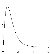
Here are two examples of F distributions. They differ in the degrees of freedom:
When the null hypothesis is rejected you conclude that the means are not all the same. But we are left with the question of which means are different:
T-Tests can't be used: We can't do this in the obvious way (using T-Tests on the various pairs of groups) because we would get too "rosy" a picture of the significance (for reasons I don't go into). The Post Hoc tests gaurantee we don't get too "rosy" a picture (actually, they provide a picture that is too "glum"!).
Two Post Hoc tests are commonly used (although ViSta doesn't offer any Post Hoc tests):
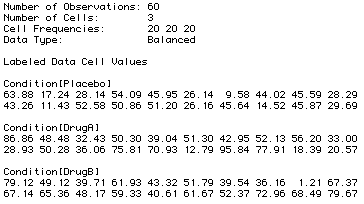
Here are the data as shown in ViSta's data report:
The data may be gotten from the ViSta Data Applet. Then, you can do the analysis that is shown below yourself.
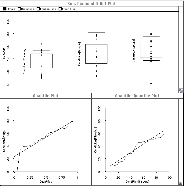
The data visualization is shown below. The boxplot shows that there is somewhat more variance in the "DrugA" group, and that there is an outlier in the "DrugB" group. The Q plots (only the "DrugB" Q-Plot is shown here) and the Q-Q plot show that the data are normal, except for the outlier in the "DrugB" group.
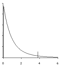
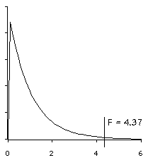
Here is the F distribution for df=2,57 (3 groups, 60 observations). I have added the observed F=4.37:

or, using the vocabulary of ANOVA,

For the data above:

(Note: The book says 11.28, but this is a rounding error. The correct value is 11.25.)
With each visualization we present the corresponding F-Test value and its p value.
Note that in these examples, the means of the three groups haven't varied, but the variances have. We see that when the groups are well separated, the F value is very significant. On the other hand, when they overlap a lot, the F is much less significant.
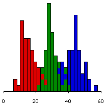
F=854.24, p<.0001.
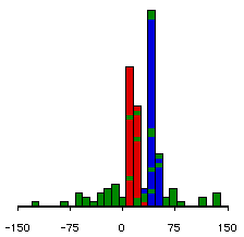
F=11.66, p<.0001.
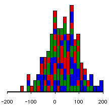
F=1.42, p=.2440.
Given these two factors, we can sketch the distribution of F-ratios. The distribution piles up around 1.00, cuts off at zero, and tapers off to the right.


Post Hoc tests help give us an answer to the question of which means are different.
Post Hoc tests are done "after the fact": i.e., after the ANOVA is done and has shown us that there are indeed differences amongst the means. Specifically, Post Hoc tests are done when:
A Post Hoc test enables you to go back through the data and compare the individual treatments two at a time, and to do this in a way which provides the appropriate alpha level.
The hypotheses, for ANOVA, are:

We arbitrarily set

The data are obtained from 60 subjects, 20 in each of 3 different experimental conditions. The conditions are a Placebo condition, and two different drug conditions. The independent (classification) variable is the experimental condition (Placebo, DrugA, DrugB). The dependent variable is the time the stimulus is endured.
We visualize the data and the model in order to see if the assumptions underlying the independent-measures F-test are met. The assumptions are:
We use ViSta to calculate the observed F-ratio, and the observed probability level.
The report produced by ViSta is shown below. The information we want is near the bottom:
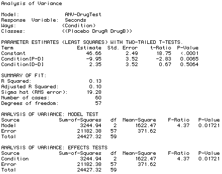
We note that F=4.37 and p=.01721. Since the observed p < .05, we reject the null hypothesis and conclude that it is not the case that all group means are the same. That is, at least one group mean is different than the others.
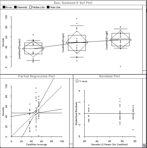
Finally, we also visualize the ANOVA model to see if the assumptions underlying the independent-measures F-test are met. The boxplots are the same as those for the data. The partial regression plot shows that the model is significant at the .05 level of significance, since the curved lines cross the horizontal line. The residual plot shows the outline in the "DrugB" group, and shows that the "DrugA" group is not as well fit by the ANOVA model as the other groups.
Here is the model visualization:
