I. Introduction to inflation

In this notes, we assume the reader is familiar with the basics of the mathematical formulation of the $\Lambda$CDM model: General Relativity (GR), Friedmann equations, cosmological horizons and the hot Big Bang in general.

Historical introduction

The inflationary theory provides the Standard Model of Cosmology with a mechanism which easily solves the horizon and flatness problems and, at the same time, it produces the primordial seeds that became the structures we see today in the sky. Independently of the nature of the mechanism, it consists on an accelerating stage of the early Universe (similar to the current one driven by the dark energy) which happened only for a brief period ―around $10^{-36}$ seconds―, soon after the Big Bang. During this time, the Universe should have exponentially increased ―inflated― by a factor of $10^{24}$ in order to fit the current observational constraints. As we shall see, the comoving Hubble radius decreases during this stage and, therefore, observable scales were inside the horizon at the beginning, i.e. in causally-connected regions. Hence, this solves the horizon problem. A similar analysis shows that the flatness problems is solved too.

Different mechanisms to inflate the universe have been proposed. The original one, due to Alan Guth, consisted in a new scalar field trapped in a false vacuum state whose energy density drives the accelerated expansion. The false vacuum is unstable and decays into a true vacuum by means of a process called quantum bubble nucleation. The hot Big Bang was then generated by bubble collisions whose kinetic energy is obtained from the energy of the false vacuum. A deep analysis of this mechanism, however, showed that this method does not work for our Universe: for sufficiently long inflation to solve the horizon problem, the bubble collision rate is not even small but it does not happen at all as the bubbles get pushed to causally disconnected regions due to the expansion. Even though Guth's mechanism did not work, he showed that an accelerated expanding universe was indeed able to solve the horizon and flatness problems.

Soon after, Andrei Linde and, independently, Andreas Albrecht and Paul Steinhardt introduced a new mechanism in which the new scalar field, instead of being trapped in a false vacuum, is rolling down a smooth potential. Inflation then takes place while the field rolls slowly compared to the expansion rate of the Universe. Once the potential becomes steeper, the field rolls towards the vacuum state, oscillates around the minimum and reheats the Universe. This new mechanism has prevailed up to now and is currently called Slow-Roll inflation.

In 1981, Viatcheslav Mukhanov and Gennady Chibisov showed an amazing consequence of an accelerated stage of the primordial universe: quantum fluctuations present during this epoch, are able to generate the primordial density perturbations, and that their spectra amplitude are consistent with observations. Later, during the 1982 Nuffield Workshop on the Very Early Universe, four different working groups, led by Stephen Hawking, Alexei Starobinsky, Alan Guth and So-Young Pi, and James Bardeen, Paul Steinhardt and Michael Turner computed the primordial density perturbations generated due to quantum fluctuations by the slow-roll mechanism. These calculations made inflation not only an artifact to solve the horizon and flatness problems, but a full testable theory able to generate the initial conditions of the $\Lambda$CDM model.

The simplified picture of inflation consists then in an accelerated epoch driven by the energy density of a new scalar field, dubbed the inflaton, which slowly rolls down its potential. Once the inflaton acquires a large velocity, inflation ends and the inflaton oscillates around the minimum of the potential, reheating the Universe i.e. giving birth to the hot Big Bang universe. During the inflaton evolution, vacuum fluctuations of the inflaton field are continuously created everywhere in space. These fluctuations, which were in thermal equilibrium, get stretched to classical levels, exiting the horizon and originating overdensity fluctuations that seeded the structure formation of the Universe.

$\Lambda$CDM problems

The $\Lambda$CDM model, consisting on different phases, each driven by very different physical processes, is able to explain with incredible accuracy a large amount of direct and indirect observations. However, it does not provide neither the initial conditions for the primordial fluid in the very early universe ―its assumed homogeneity and isotropy― nor the required density perturbations which are the seeds for the structures we observe today in our Universe; these ingredients are just assumed to be there.

On one hand, it is indeed a puzzle the homogeneity observed in the Universe. Take for instance the CMB anisotropies. The differences in temperature are of order of $10^{-5}$, however, the CMB consists of $10^4$ causally disconnected patches which have never been in thermal equilibrium. How do they have the same temperature then? ―Horizon problem―. On the other hand, for our universe to be flat now, it must have been flat to an incredibly degree in the far past, a value uncomfortably small to take as an initial condition ―flatness problem―. These two issues are the main problems of the standard model of Cosmology.

Horizon problem

The particle horizon can be written as $$ \label{eq:horprob} \tau=\int_0^{a'}\frac{\text{d}\text{ln} a}{aH}~. $$ Furthermore, one can use the definition $\text{d} t=a\text{d}\tau$ and find that the combination $(aH)^{-1}$ grows, for a matter (with $\omega=0$)- or radiation (with $\omega=-1/3$)-dominated universe, as $$ \left(aH\right)^{-1}\propto a^{\frac12\left(1+3\omega\right)}~, $$ and therefore the particle horizon \eqref{eq:horprob} grows in a similar way.

The quantity defined as $(aH)^{-1}$ is called the comoving Hubble radius, and its implications are quite important: as the comoving Hubble radius has been growing monotonically with time during the evolution of the Universe, observable scales are now entering the particle horizon and, therefore, they were outside causal contact in the far past, at the CMB decoupling for instance. Consequently, the homogeneity problem is manifest: around $10^4$ causally disconnected patches over the observable sky have never been in thermal equilibrium and yet they have almost exactly the same temperature!

Flatness problem

We have now defined the comoving Hubble radius, which clearly is a function of time that monotonically grows during the evolution of the Universe. From the Friedmann equation, $$ |\Omega(a)-1|=\biggr|\frac{k}{(aH)^2}\biggr|~, \label{eq:flatness2} $$ where we recall that $\Omega(a)\equiv\rho(a)/\rho_c(a)$. Because $(aH)^{-1}$ grows with time, $|\Omega(a)-1|$ must diverge and therefore the value $\Omega(a)=1$ is an unstable fixed point, as seen from the differential equation

$$ \diff{\ln \Omega}{\ln a}=\mk{1+3\omega}\mk{\Omega-1}~.$$ For the observed value $\Omega(a)\sim1$, the initial conditions for $\Omega$ then require an extreme fine tuning. For instance, to account for the flatness today, $|\Omega(a_\text{BBN})-1|\leq\mathcal{O}\mk{10^{-16}}$ or $|\Omega(a_\text{GUT})-1|\leq\mathcal{O}\mk{10^{-61}}$. Setting then those orders of magnitude as initial conditions imply a huge fine-tuning problem.

Initial perturbations problem

Finally, even though the homogeneity and isotropy is evident, it is not perfect. There exist structures like galaxies, cluster of galaxies and cosmic voids which back in time were seeded by small density perturbations which differed in amplitude by $\delta\rho/\rho\sim10^{-5}$, according to the level of anisotropy observed in the CMB produced at the recombination epoch. These perturbations are, again, assumed and put "by hand", as the $\Lambda$CDM model has no mechanism which can produce them. To thad end, a theory providing a mechanism for the generation of these primordial seeds is very appealing.

In the following, we shall see that both the horizon and flatness problems are trivially solved if we account for an epoch in which the cosmological Hubble radius decreases before starting to increase again, and that this epoch must consist in an accelerated expansion of the Universe. Furthermore, in the quantum regime, vacuum fluctuations subject to this accelerated expansion could be stretched to classical scales, becoming into the primordial seeds we are looking for. Such a mechanism is now conceived as inflation (for reasons we are about to discuss) and it is not only and artifact to solve the horizon and flatness problem, but a theory where the laws of GR and those of quantum mechanics are put to work together, converting inflation in the theory of the primordial quantum fluctuations.

$\Lambda$CDM problems revisited

As already pointed out, the heart of the $\Lambda$CDM problems is the growing nature of the comoving Hubble radius $\left(aH\right)^{-1}$ ―a region enclosing events that are causally-connected at a given time― during the evolution of the Universe. As a consequence, most of the observable scales must have been disconnected in the past. The intuitive solution is then a mechanism which makes the comoving Hubble radius decrease during the early times. This would imply that observable scales were causally-connected at some initial time and then exited the horizon when it decreased. The horizon problem would then be solved as causally-connected regions would have been allowed to be in thermal equilibrium.

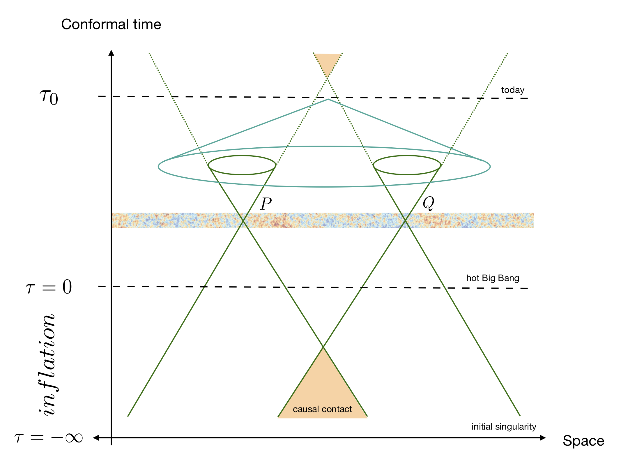
During inflation, the Hubble parameter $H$ is approximately constant. Therefore, the particle horizon $\tau$, given by Eq. \eqref{eq:horprob}, can be integrated explicitly as $$ \tau\simeq-\frac{1}{aH}~. $$ So one can see that a large past Hubble horizon $\left(aH\right)^{-1}$ would make $\tau$ fairly large today, making it larger than the present Hubble horizon $\left(a_0H_0\right)^{-1}$, i.e. two largely-separated points in the CMB would not communicate today but would have in the past if they are inside the particle horizon. The figure below sketches this reasoning.

Figure 1: Evolution of the comoving Hubble radius $\left(aH\right)^{-1}$. At early times, the horizon was large enough so that observable scales were in causal contact. As inflation took place, the horizon shrank and scales came out to disconnected regions. Inflation then finished and the horizon started to grow to the present size. Two casually-disconnected CMB points, $P$ and $Q$, were then in thermal equilibrium at some point in the past, thus resolving the horizon problem.

Furthermore, it is evident from Eq. \eqref{eq:flatness2} that a decreasing Hubble radius drives the Universe towards flatness, and just deviating from it at present times. Thereby $\Omega=1$ went from being an unstable fix point to be an attractor solution thanks to inflation, thus also solving the flatness problem.

Conditions for inflation

The shrinking Hubble radius entails important consequences for the evolution of the scale factor $a$, i.e. for the evolution of the Universe. First, lets note that the change of the decreasing $\mk{aH}^{-1}$ over time is $$ \diff{}{t}\mk{\f{1}{aH}}=-\f{\ddot a}{\mk{aH}^2}<0~,$$ and therefore, from the inequality, $$ \ddot a>0~, \label{eq:adotdot} $$ is a necessary condition for the shrinking of the Hubble radius. It is evident then that we require an accelerated expansion to solve the horizon and flatness problems!

Furthermore, Eq. \eqref{eq:adotdot} has implications on the evolution of the Hubble parameter due to their relation $\dot H=(\ddot a/a)-H^2$, and hence $$ \f{\ddot a}{a}=H^2\mk{1-\epsilon_H}~, $$ where we have defined the first slow-roll parameter as $$ \epsilon_H\equiv-\f{\dot H}{H^2}<1~. \label{eq:epsilonh} $$ As we shall see, $\epsilon_H$ is one of the most important parameters in inflation, as it quantifies its duration and, equivalently, determines when it finishes.

Furthermore, from the second Friedmann equation, $$ \begin{align} \f{\ddot a}{a}=H^2\mk{1-\epsilon_H}&=-\frac16\mk{\rho+3p}\\ &=-\frac\rho6\mk{1+3\omega}~, \label{eq:epome} \end{align} $$ where, for $\epsilon_H\to0$ and a flat Universe with $\rho=\rho_c=3H^2$, we find that Eq. \eqref{eq:epome} leads to $$ \omega\to-1~, \qquad \leftrightarrow \qquad a\propto e^{Ht}~. $$ This means that the expansion increases exponentially or, in other words, the universe inflates! In a general case, Eq. \eqref{eq:epome} suggests a more general condition for inflation: $$ p<-\frac13\rho~, $$ which implies that the accelerated expansion is driven by a fluid with negative pressure.

Finally, notice that Eq. \eqref{eq:epsilonh} shows that during this accelerated expansion, the rate of change of the Hubble parameter is small, meaning that $H$ is approximately constant during inflation. This has important consequences on the conformal time; namely $$ \tau=-\frac{1}{aH}~, \qquad \leftrightarrow \qquad a=-\f{1}{H\tau}~, $$ and therefore the singularity $a=0$ is pushed to $\tau\to-\infty$ . Consequently, at $\tau=0$ the scale factor is not well defined and inflation must end before reaching this epoch ($H\sim const.$) stops being a good approximation). The spacetime defined with these characteristics is called de Sitter space and it is exactly the spacetime of inflation. To see the consequences of this in the evolution of two CMB points, let us take Fig. 1 and put it in perspective as a function of the conformal time $\tau$, shown in Fig 2. If we take only the period containing the hot Big Bang (from $\tau=0$ to $\tau_0$), two CMB points could have never been in contact, whereas once we assume inflation took place, the light cones of these two points intersect in the far past, allowing them to be in thermal equilibrium.

Figure 2: Conformal diagram including the inflationary epoch. Inflation, pushes the initial singularity to an arbitrary point in the past ($\tau=-\infty$) allowing the light cones of two CMB points, $P$ and $Q$, which are causally disconnected now, to be in thermal equilibrium at some point in the past, thus solving the horizon problem.

Before continuing, and to summarize, let us emphasize that whatever the mechanism for inflation is, the simple fact that the comoving Hubble radius shrinks implies that the following conditions must be (mutually) satisfied: $$ \ddot a>0~, \qquad \epsilon_H\equiv-\f{\dot H}{H^2}<1~, \qquad p<-\frac13\rho~. \label{eq:condforinf} $$ Now, let us discuss in Lecture II how the energy density of a scalar field driving inflation, subject to the slow-roll approximation, effectively satisfies these conditions.