Definition: The Pearson correlation measures the degree and direction of a linear relationship between two variables.
Notation: The Pearson correlation is denoted by the letter r.
- Conceptual Formula
- Sum of Products of Deviations :
- The Algebraic Formula :
- Z-Scores and Pearson Correlation :
Conceptually, the Pearson Correlation is the ratio of the variation shared by X and Y to the variation of X and Y separately. The conceptual formula is:

Stated in statistical terminology:

When there is a perfect linear relationship, every change in the X variable is accompanied by a corresponding change in the Y variable. In this case, all variation in X is shared with Y, so the ratio given above is r=1.00. At the other extreme, when there is no linear relationship between X and Y, then the numerator is zero, so r=0.00.
To calculate the Pearson correlation, it is necessary to introduce one new concept: The sum of the products of corresponding deviation scores for two variables. We have already seen a similar concept, the sum of the squares of the deviation scores for a variable.
The sum of squares, which is used to measure the amount of variability of a single variable, is defined as:

The sum of products, which is used to measure the variability shared between two variables, is defined as:

Note that the name is short for the sum of the products of corresponding deviation scores for two variables.
To calculate the SP, you first determine the deviation scores for each X and for each Y, then you calculate the products of each pair of deviation scores, and then (last) you sum the products.
As noted above, conceptually the Pearson correlation coefficient is the ratio of the joint covariability of X and Y, to the variability of X and Y separately. The formula uses the SP as the measure of covariability, and the square root of the product of the SS for X and the SS for Y as the measure of separate variability. That is:

If we have scores that are expressed as standardized scores -- Z-Scores with a mean of zero and a variance of one -- then the formula for the Pearson Correlation becomes particularly simple. It is:

- Correlation is NOT Causation!
- Correlation and Restricted Range
- Outliers (Outriders?)
- Correlation and Strength of Relationship
- The Coefficient of Determination:
- The Coefficient of Determination, which is the squared correlation coefficient, measures the percentage of variation shared between the two variables.
One of the most common errors made in interpreting correlations is to assume that a correlation necessarily implies a cause-and-effect relationship between the two variables. Simply stated: Correlation is NOT Causation!
When a correlation is computed from scores with a restricted range the correlation coefficient is lower than it would be if it were computed from scores with an unrestricted range.
This happens when we look at the correlation between SAT and GPA among students in this class, since we are only seeing those students who were admitted to UNC. Those with low SAT scores (who presumably would have had very low GPA scores) were not admitted. Thus, we have a restricted range of observed SAT scores, and a lower correlation.
For example, consider the relationship between Automobile weight and Horsepower shown in the following scatterplot:
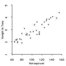
If we lived in a country that restricted cars to have no more than 100 Hp, then the data would be cut off like this:
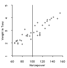
What we would see as the relationship would be only based on the cars with less than 100 HP. We would see:
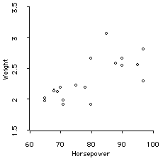
Now the correlation is only .71, rather than .92.
Outliers (which G&W call, for some unknown reason, outriders) are an individual observation that has very large values of X and Y relative to all the other values of X and Y. For example, in this scatterplot of the Market Value of many companies plotted versus their Assets, the fact that IBM is so large compared to any other company completely obscures the relationship of the two variables to each other.
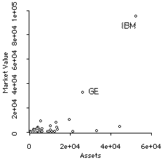
The correlation for these variables is .68, which is spuriously high. In fact, the correlation is reduced to .48 when IBM is removed.
The Pearson correlation measures the degree of relationship between two variables. It is not, however, interpreted as a percentage. On the other hand:
The basic question answered by the hypothesis testing procedure for the Pearson correlation coefficient is whether it is significantly different from zero: i.e., whether or not a non-zero correlation exists in the population. Here are the four standard hypothesis testing steps, as augmented by a visualization step for the data:
- State the hypotheses
- Set the decision criterion
- Gather the data
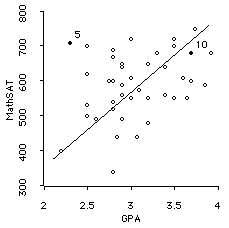
- The MathSAT/GPA correlation is .32 -- 10% of the variance in GPA is explained by MathSAT.
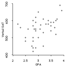
- The VerbalSAT/GPA correlation is .47 -- 22% of the variance in GPA is explained by VerbalSAT.
- Remember that these correlations have been attenuated by restriction of range.
- If we had a larger sample, and these correlation values stayed about the same, then they would become significant. However, significance isn't everything, as the size of the correlation tells us how strong the relationship is.
- Visualize the data
- Evaluate the Hypothesis
- For df = 35 the critical r = .275.
- For df = 40 the critical r = .257.
Thus - For df = 39 the critical r
= .275 - (.275 - .257)*(4/5)
= .275 - .014
= .261
The hypotheses concern whether or not there exists a non-zero correlation in the population. We have a 1-tailed hypothesis:

There are also two possible 1-tailed hypothesis. Here's one of them:

Choose an alpha level.
The df=n-2, where n is the number of pairs.
Lets use the data gathered in class about SAT-M and GPA. We can also use the SAT-V and GPA correlation. We observe that
Here are the two scatterplots:
 | 
|
For df=39, alpha=.05, we can interpolate to find the the critical one-tailed r.
Therefore, for both relationships, we reject the null hypothesis that there is not a positive correlation in the population (in plain English, we say these correlations are significantly different from zero). The two SAT scales DO significantly predict your GPA's.
The ViSta Applet demonstrates that you can compute Pearson correlations in two ways:
- Summarize Data You can get a report of correlations among the active numeric variables by choosing the Data menu's Summarize Data item and then clicking on the Correlation Matrix check box. The report will contain a matrix of correlations.
- Transform You can compute a data object containing correlations by choosing the Transform menu's Correlations item. A data object containing a matrix of correlations among the active numeric variables will be created.
The commands to do this are:
(browse-data)
(summarize-data :moments t :correlations t)
(correlations)
(browse-data)