3.2.5 Prelude to nonlinear problems

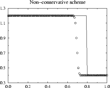
For non-linear problems, to be discussed later, the solution can develop discontinuities after a finite time even if the initial data are smooth

The way to handle properly discontinuous solutions and to converge to the physical solution is to use numerical schemes written in conservation form

$\begin{displaymath} u_j^{n+1} = u_j^n - \frac{\Delta t}{\Delta x} \left(\hat{f}_{j+\frac{1}{2}} - \hat{f}_{j-\frac{1}{2}}\right) \end{displaymath}$

(78)

Let us consider the Burger's equation with discontinuous initial data

$\begin{displaymath} \frac{\partial u}{\partial t} + \frac{\partial (\frac{1}{2}u^2)}{\partial x} = 0 \end{displaymath}$

(79)

It can be discretized by the upwind conservative method

$\begin{displaymath} u_j^{n+1} = u_j^n - \frac{\Delta t}{\Delta x} \left(\frac{1}{2}(u_j^n)^2 - \frac{1}{2}(u_{j-1}^n)^2 \right) \end{displaymath}$

(80)

$\begin{figure}\centerline{\psfig{figure=../FIGURES_DATABASE/cons.eps,width=10cm}}\end{figure}$

On the other hand, one could discretize the quasilinear form of Burger's equation

$\begin{displaymath} \frac{\partial u}{\partial t} + u\frac{\partial u}{\partial x} = 0 \end{displaymath}$

(81)

using the nonconservative upwind method

$\begin{displaymath} u_j^{n+1} = u_j^n - \frac{\Delta t}{\Delta x}u_j^n \left(u_j^n - u_{j-1}^n \right) \end{displaymath}$

(82)

$\begin{figure}\centerline{\psfig{figure=../FIGURES_DATABASE/noncons.eps,width=10cm}}\end{figure}$