Next: 3.3.1 Weak solutions Up: 3 Sistemas Hiperbólicos de Previous: 3.2.5 Prelude to nonlinear
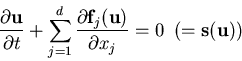
Let us consider the system of ![]() equations of conservation laws
equations of conservation laws
Formally, system (84) expresses the conservation of the vector
![]() . Let
. Let ![]() be an arbitrary domain of
be an arbitrary domain of ![]() and let
and let
![]() the outward unit normal to the boundary
the outward unit normal to the boundary ![]() of
of
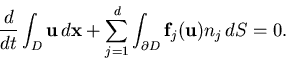
![]() . Then, from (84), it follows that
. Then, from (84), it follows that
 is equal to the losses
through the boundary
is equal to the losses
through the boundary
Now, for all ![]() let
let
| (85) |
Definition:
The system (84) is called hyperbolic if,
for any ![]() and any
and any
![]() , the matrix
, the matrix
 |
(86) |
In most situations we will consider the so-called
initial value problem (IVP), i.e., the solution of
system (84) with the initial condition
A key property of hyperbolic systems is that features in the solution
propagate at the characteristic speeds given by the
eigenvalues of the
Jacobian matrices. The characteristic curves associated to system
(84) are the integral curves of the differential equations
| (88) |
Continuous and differentiable solutions that satisfy (84) and
(88) pointwise are called classical solutions.
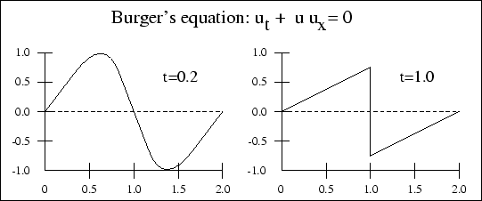
However, for
non-linear systems, classical solutions do not exist in general even when the
initial condition ![]() is a smooth function, and
discontinuities develop after a finite time.
is a smooth function, and
discontinuities develop after a finite time.
Then we seek generalized solutions that satisfy the integral form of the conservation system (85) which are classical solutions where they are continuous and have a finite number of discontinuities (weak solutions)