- Objects
- Read a
Windowof data - Read a
Windowfrom the raster object - Conversions
- Change of Refence System (
CRS) usingrasterio.warp - Crop raster with a polygon (
listof coordinates) - Reproject raster to different
CRS
(See this post in notebook format)
This blog post is a tutorial/show case of the python package rasterio. In particular I have focused on select specific parts of a raster based on a list of coordinates, squared shapes (bounding boxes) or polygons. We will deal with the different conversions between different objects rasterio uses for this and how to go from one to another. Afterwards I will show you how to show this shapes in an open street maps map using folium and how to reproject the a region within the raster to a different coordinate system.
I will use a Sentinel 2 Level 2 image saved as 4 band geotiff for the examples. This image is projected in a regular grid in the UTM coordinate reference system. Here there is a similar example using Landsat 8 images which can be downloaded directly with rasterio.
The first code snippet after the imports load the geotiff metadata and shows the shape of the image together with the Affine transformation and the coordinate reference system (epsg:32630 which corresponds to UTM zone 30N). Coordinate reference systems in rasterio are encoded within the class rasterio.crs.CRS.
Objects
There is a pletora of objects that rasterio defines to deal with change of coordinates, squared regions and polygons. We will focus in the following list and we will later see how can we move from one to another:
Window. AWindowis a square region of an image given in (row,col) coordinates (image coordinates).BoundingBox. ABoundingBoxis a square region of an image given in coordinates (in coordinates from an specific coordinate reference system (CRS))listof indexes (row,col).listof pixels indexes within an image.listof coordinates*.listof coordinates (x,y) in a given coordinate reference system (CRS).shapely.PolygonandGeoJSONlikedictionary. Polygons are list of coordinates that form a closed polygon in the plane.shapelyis a python module that allow to easily compute intersections and unions of polygons and other type of shapes.GeoJSONlikedictionaryis a format to encode vector data widely used in the Internet. I is also used byrasterioto deal with polygon objects. We will see that in its most basic form is a simple pythondictiorarywith two fields:typeandcoordinates.
import rasterio
from rasterio.coords import BoundingBox
from rasterio import windows
from rasterio import warp
from rasterio import mask
import numpy as np
import folium
import matplotlib.pyplot as plt
import rasterio.plot as plot
from matplotlib.patches import Rectangle
src = rasterio.open('/path/to/s2/image/S2_image_flat.tif')
print(src.height,src.width,src.transform,src.crs)
10980 10980 | 10.00, 0.00, 300000.00|
| 0.00,-10.00, 4700040.00|
| 0.00, 0.00, 1.00| +init=epsg:32630
With the Affine transform we can shift between (row,col) coordinates within the image to (x,y) epsg:32630 coordinates. We will see this later here.
Read a Window of data
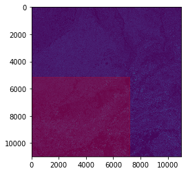
A Window is a square region of an image given in image coordinates (row,col). We can create a Window object from a tuple of slice objects. As we can see, this window selects the pixels form row 5150 to src.height and cols from 0 to 7168. The following snippet shows the first band of the image and the selected rectangle in red.
slice_ = (slice(5150,src.height),slice(0,7168))
window_slice = windows.Window.from_slices(*slice_)
print(window_slice)
Window(col_off=0, row_off=5150, width=7168, height=5830)
datos_b1 = src.read(1)
plt.imshow(datos_b1)
ax = plt.gca()
ax.add_patch(Rectangle((window_slice.col_off,window_slice.row_off),
                       width=window_slice.width,
                       height=window_slice.height,fill=True,alpha=.2,
                 color="red"))
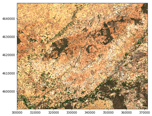
Read a Window from the raster object
We will plot the raster Window using rasterio.plot. Notice that in order to show the coordinates appropriately we must find the specific Affine transform of the Window (which consists just in shifting the origin of the original src.transform).
# find specific transform, necessary to show the coordinates appropiately
transform_window = windows.transform(window_slice,src.transform)

# Read img and convert to rgb
img = np.stack([src.read(4-i, window=window_slice) for i in range(1,4)],
               axis=-1)
img = np.clip(img,0,2200)/2200

print(img.shape)
plt.figure(figsize=(8,8))
plot.show(img.transpose(2,0,1),
          transform=transform_window)
(5830, 7168, 3)
# Useful functions

def reverse_coordinates(pol):
    """
    Reverse the coordinates in pol
    Receives list of coordinates: [[x1,y1],[x2,y2],...,[xN,yN]]
    Returns [[y1,x1],[y2,x2],...,[yN,xN]]
    """
    return [list(f[-1::-1]) for f in pol]

def to_index(wind_):
    """
    Generates a list of index (row,col): [[row1,col1],[row2,col2],[row3,col3],[row4,col4],[row1,col1]]
    """
    return [[wind_.row_off,wind_.col_off],
            [wind_.row_off,wind_.col_off+wind_.width],
            [wind_.row_off+wind_.height,wind_.col_off+wind_.width],
            [wind_.row_off+wind_.height,wind_.col_off],
            [wind_.row_off,wind_.col_off]]

def generate_polygon(bbox):
    """
    Generates a list of coordinates: [[x1,y1],[x2,y2],[x3,y3],[x4,y4],[x1,y1]]
    """
    return [[bbox[0],bbox[1]],
             [bbox[2],bbox[1]],
             [bbox[2],bbox[3]],
             [bbox[0],bbox[3]],
             [bbox[0],bbox[1]]]

def pol_to_np(pol):
    """
    Receives list of coordinates: [[x1,y1],[x2,y2],...,[xN,yN]]
    """
    return np.array([list(l) for l in pol])

def pol_to_bounding_box(pol):
    """
    Receives list of coordinates: [[x1,y1],[x2,y2],...,[xN,yN]]
    """
    arr = pol_to_np(pol)
    return BoundingBox(np.min(arr[:,0]),
                       np.min(arr[:,1]),
                       np.max(arr[:,0]),
                       np.max(arr[:,1]))
Conversions
Next sections will cover the conversions of our window to different objects types.
Window to list of index (row,col)
pol_index = to_index(window_slice)
pol_index
[[5150, 0], [5150, 7168], [10980, 7168], [10980, 0], [5150, 0]]
Convert list of index (row,col) to list of coordinates
To obtain the coordinates of a list of (row,col) pairs we can directly multiply them by the src.transform object (from class Affine). However a couple of things must be taken into account: first the src.transform object transforms (col,row) coordinates (instead of (row,col)) so we must reverse our coordinates before multiplying. In addition, the multiplication returns the coordinates of the upper left (ul) pixel, therefore if we want the coordinates of the center pixel we should add .5 to each of our (row,col) pairs.
We can also use the build-in method xy from the raster object.
[list(src.transform*p) for p in reverse_coordinates(pol_index)]
[[300000.0, 4648540.0],
 [371680.0, 4648540.0],
 [371680.0, 4590240.0],
 [300000.0, 4590240.0],
 [300000.0, 4648540.0]]
[list(src.xy(*p,offset="center")) for p in pol_index]
[[300005.0, 4648535.0],
 [371685.0, 4648535.0],
 [371685.0, 4590235.0],
 [300005.0, 4590235.0],
 [300005.0, 4648535.0]]
[list(src.xy(*p,offset="ul")) for p in pol_index]
[[300000.0, 4648540.0],
 [371680.0, 4648540.0],
 [371680.0, 4590240.0],
 [300000.0, 4590240.0],
 [300000.0, 4648540.0]]
Convert Window to BoundingBox
bbox = windows.bounds(window_slice,src.transform)
bbox
(300000.0, 4590240.0, 371680.0, 4648540.0)
Convert BoundingBox to Window
window_same = windows.from_bounds(*bbox,src.transform)
window_same
Window(col_off=0.0, row_off=5150.0, width=7168.0, height=5830.0)
BoundingBox to list of coordinates (closed)
pol = generate_polygon(bbox)
pol
[[300000.0, 4590240.0],
 [371680.0, 4590240.0],
 [371680.0, 4648540.0],
 [300000.0, 4648540.0],
 [300000.0, 4590240.0]]
list of coordinates to BoundingBox
pol_to_bounding_box(pol)
BoundingBox(left=300000.0, bottom=4590240.0, right=371680.0, top=4648540.0)
Change of Refence System (CRS) using rasterio.warp
We will change the reference system from the different types of objects we have generated so far. The source reference system of our raster is UTM epsg:32630. The target reference system we will use is epsg:4326 which corresponds to standard (longitude,latitude) coordinates. Transformations are done using the rasterio.warp module. There are different functions depending on the objects we want to transform to.
transform list of coordinates
pol_np = np.array(pol)
coords_transformed = warp.transform(src.crs,{'init': 'epsg:4326'},pol_np[:,0],pol_np[:,1])
coords_transformed = [[r,c] for r,c in zip(coords_transformed[0],coords_transformed[1])]
coords_transformed
[[-5.393939163550343, 41.4388362850582],
 [-4.536330188462325, 41.453491755554914],
 [-4.548885155675175, 41.97841583786727],
 [-5.413488998912444, 41.963489431071004],
 [-5.393939163550343, 41.4388362850582]]
transform BoundingBox
bounds_trans = warp.transform_bounds(src.crs,{'init': 'epsg:4326'},*bbox)
print(bounds_trans)
pol_bounds_trans = generate_polygon(bounds_trans)
pol_bounds_trans
(-5.413488998912444, 41.4388362850582, -4.536330188462325, 41.97841583786727)

[[-5.413488998912444, 41.4388362850582],
 [-4.536330188462325, 41.4388362850582],
 [-4.536330188462325, 41.97841583786727],
 [-5.413488998912444, 41.97841583786727],
 [-5.413488998912444, 41.4388362850582]]
transform GeoJSON like dictionary
A GeoJSON like dictionary in its simplest form is a dictionary with a a field type set to Polygon and a field coordinates as a list of list of coordinates. The function warp.transform_geom use this structure to transform geometries between different coordinate reference systems (CRS).
pol_trans = warp.transform_geom(src.crs,{'init': 'epsg:4326'},
                                {"type":"Polygon","coordinates":[pol]})
pol_trans
{'type': 'Polygon',
 'coordinates': [[(-5.393939163550343, 41.4388362850582),
   (-4.536330188462325, 41.453491755554914),
   (-4.548885155675175, 41.97841583786727),
   (-5.413488998912444, 41.963489431071004),
   (-5.393939163550343, 41.4388362850582)]]}
As we can see, pol_trans and coords_transformed are the same but not the transformed coordinates of BoundingBox (generate_polygon(bounds_trans)). That is because a BoundingBox is a rectangle with axes parallel to the used CRS. We will see this graphically in the next section. In addition, we could get the same BoundingBox if we use the pol_to_bounding_box function.
pol_to_bounding_box(pol_trans["coordinates"][0])
BoundingBox(left=-5.413488998912444, bottom=41.4388362850582, right=-4.536330188462325, top=41.97841583786727)
Show polygons with folium
Now we will show all the polygons we have defined using folium. In particular we will show the bounds of the original image, the polygons of the transformed coordinates (and we will see they are both the same) and the bounds of the transformed window. With the functions folium.Polygon and folium.Polyline we can easily plot in an OpenStreetMap map our list of coordinates. However we should reverse the coordinates in such lists because folium works with (lat,lng) coordinates instead of (lng,lat).
# original bounds of the image
bounds_trans_original = warp.transform_bounds(src.crs,{'init': 'epsg:4326'},
                                              *src.bounds)
polygon_trans_original = generate_polygon(bounds_trans_original)

polyline_polygon_trans_original = folium.PolyLine(reverse_coordinates(polygon_trans_original),
                                                  popup="polygon_trans_original",
                                                  color="#2ca02c")

polyline_pol_trans = folium.Polygon(reverse_coordinates(pol_trans["coordinates"][0]),
                                    popup="pol_trans",color="red",fill=True)

polyline_coords_transformed = folium.PolyLine(reverse_coordinates(coords_transformed),
                                              popup="coords_transformed")

# transformed bounds which should be different than the previous two
polyline_pol_bounds_trans = folium.PolyLine(reverse_coordinates(pol_bounds_trans),
                                            popup="pol_bounds_trans",color="orange")

mean_lat = (bounds_trans[1] + bounds_trans[3]) / 2.0
mean_lng = (bounds_trans[0] + bounds_trans[2]) / 2.0
map_bb = folium.Map(location=[mean_lat,mean_lng],
                zoom_start=6)
map_bb.add_child(polyline_pol_trans)
map_bb.add_child(polyline_coords_transformed)
map_bb.add_child(polyline_pol_bounds_trans)
map_bb.add_child(polyline_polygon_trans_original)
map_bb
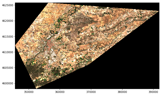
Crop raster with a polygon (list of coordinates)
It is very common that we are just interested in an specific region within a raster given by the a polygon (list of coordinates). To just keep that region of the raster and get rid of the rest the simplest option is to use rasterio.mask.mask (see: masking raster using a shapefile).
First we define our polygon of the region of interest (RoI):
roi_polygon = [[-4.853330696593957,41.64565614198989],
               [-4.768186653625207,41.522392372903866],
               [-4.569059456359582,41.59432483529684],
               [-4.30,41.75229435821611],
               [-4.728361214172082,41.77073301997901],
               [-4.853330696593957,41.64565614198989]]
Then we transform the (RoI) which is given in long/lat coordinates to the raster coordinates (which are given in src.crs coords). Then, with the polygon defined as a GeoJSON like dictionary we call rasterio.mask.mask. (Watch out this function work with a list of GeoJSON like dictionary and if you pass it just a single dictionary it raises an error).
roi_polygon_src_coords = warp.transform_geom({'init': 'epsg:4326'},
                                             src.crs,
                                             {"type": "Polygon",
                                              "coordinates": [roi_polygon]})

out_image,out_transform = mask.mask(src,
                                    [roi_polygon_src_coords],
                                    crop=True)

out_image = np.clip(out_image[2::-1],
                    0,2200)/2200

plt.figure(figsize=(10,10))
plot.show(out_image,
          transform=out_transform)
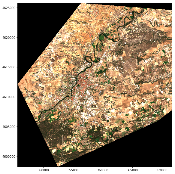
Intersect our window with the defined polygon
Great! so now suppose you are interested only in the intersection between the roi_polygon and our previously defined window. In this case we can use shapely to compute the intersection. Once we have the intersected polygon we proceed as we did before.
from shapely.geometry import Polygon

pol_intersection = Polygon(pol_trans["coordinates"][0]).intersection(Polygon(roi_polygon))
pol_intersection = [list(l) for l in list(pol_intersection.exterior.coords)]
pol_intersection
[[-4.5437277787345245, 41.76278553698213],
 [-4.54010517941412, 41.61132439880385],
 [-4.569059456359582, 41.59432483529684],
 [-4.768186653625207, 41.522392372903866],
 [-4.853330696593957, 41.64565614198989],
 [-4.728361214172082, 41.77073301997901],
 [-4.5437277787345245, 41.76278553698213]]
map_bb.add_child(folium.PolyLine(reverse_coordinates(pol_intersection),
                                 color="#999999"))
map_bb.add_child(folium.PolyLine(reverse_coordinates(roi_polygon),
                                 color="#222222"))
map_bb
pol_intersection_src_coords = warp.transform_geom({'init': 'epsg:4326'},
                                                  src.crs,
                                                  {"type": "Polygon",
                                                   "coordinates": [pol_intersection]})
out_image,out_transform = mask.mask(src,
                                    [pol_intersection_src_coords],
                                    crop=True)

out_image = np.clip(out_image[2::-1],
                    0,2200)/2200

plt.figure(figsize=(10,10))
plot.show(out_image,
          transform=out_transform)
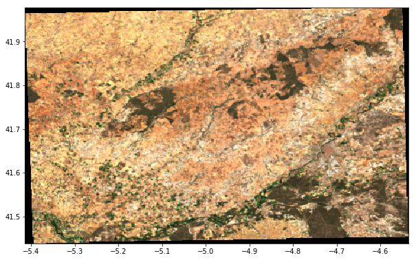
Reproject raster to different CRS
In this section we are going to show how to change the coordinates of the raster window we showed in section 3. In particular we want to reproject it to the long/lat reference system and to upscale it (i.e. make its pixels bigger so that the image is smaller). Afterwards we overlay the raster in the OpenStreetMap map.
In order to change the coordinate reference system of a raster we will use the functions warp.reproject and warp.calculate_default_transform ref from the docs. The function warp.reproject takes (in the most basic form) 6 inputs:
- The source
CRS - The source
Affinetransform - The raster either (either defined as a
numpyarray or as arasterioraster) - The target
CRS - The target
Affinetransform - The target object where we want to put the reprojected raster (the
numpyorrasterioobject)
Normally we know the first 4 parameters (all related to our raster and the target CRS) however the last two we sometimes don’t know; specifically we normally don’t know what is going to be the number of rows and columns of the target array. To solve this problem we can use the warp.calculate_default_transform function, which computes the target Afinne transform and the target width and height of the target array. As inputs this function takes the source and target CRS, the width and height of the source array and the BoundingBox of the raster. In the example we use the additional parameter resolution to shrink the shape of the target raster.
transform,width,height = warp.calculate_default_transform(src.crs, {"init":"epsg:4326"},
                                                          img.shape[1],img.shape[0],
                                                          left=bbox[0],bottom=bbox[1],
                                                          right=bbox[2],top=bbox[3],
                                                          resolution=0.002)
out_array = np.ndarray((img.shape[2],height,width),dtype=img.dtype)

warp.reproject(np.transpose(img,axes=(2,0,1)),
               out_array,src_crs=src.crs,dst_crs={"init":"epsg:4326"},
               src_transform=transform_window,
               dst_transform=transform,resampling=warp.Resampling.bilinear)

plt.figure(figsize=(10,8))
plot.show(out_array,
          transform=transform)
Show the raster on an OpenStreetMap map
Finally to overlay the raster in the map we will use folium.raster_layers.ImageOverlay:
polyline_polygon_trans_original = folium.PolyLine(reverse_coordinates(polygon_trans_original),
                                                  popup="polygon_trans_original",
                                                  color="#2ca02c")

polyline_pol_trans = folium.PolyLine(reverse_coordinates(pol_trans["coordinates"][0]),
                                    popup="pol_trans",color="blue")

polyline_pol_bounds_trans = folium.PolyLine(reverse_coordinates(pol_bounds_trans),
                                            popup="pol_bounds_trans",color="orange")

mean_lat = (bounds_trans[1] + bounds_trans[3]) / 2.0
mean_lng = (bounds_trans[0] + bounds_trans[2]) / 2.0
map_bb = folium.Map(location=[mean_lat,mean_lng],
                zoom_start=8)
map_bb.add_child(polyline_pol_trans)
map_bb.add_child(polyline_pol_bounds_trans)
map_bb.add_child(polyline_polygon_trans_original)
image_overlay = folium.raster_layers.ImageOverlay(np.transpose(out_array,(1,2,0)),
                                                  [[bounds_trans[1],
                                                    bounds_trans[0]],
                                                   [bounds_trans[3],
                                                    bounds_trans[2]]])
map_bb.add_child(image_overlay)
map_bb