Deep Neural Networks as Gaussian Processes

• Introduction
• The standard Bayesian approach
  • Bayesian linear regression (standard approach)
  • Neural networks (standard approach)
• The $\mathcal{GP}$ approach
  • Bayesian linear regression ($\mathcal{GP}$ approach)
  • $\mathcal{GP}$ Regression ($\mathcal{GP}$ approach)
  • Neural networks ($\mathcal{GP}$ approach)
• Bonus track: $\mathcal{GP}$ Regression (standard Bayesian approach)

We were recently discussing the paper Deep Neural Networks As Gaussian Processes (ICLR’18) where the authors propose a Gaussian Process model that is equivalent to a fully connected deep neural network with infinite number of hidden units in each layer. They call this model: NNGP. It took me a while to understand the paper and to place this model in the context of other Bayesian approaches to neural networks. What I found out is that the paper approaches neural networks following a GP approach and that other models (linear regression and a GP regression) can also be derived using either a standard Bayesian approach or a GP approach. I found this relation very interesting and I think it could be very helpful to understand other models/papers.

Introduction

Let’s consider a regression problem. We want to find a function $f$ that map vectors $x\in\mathbb{R}^{d_{in}}$ to values $y\in\mathbb{R}$. For this problem, the most common probabilistic model to use is:

\[\begin{aligned} y_i &= f(x_i) + \epsilon_i\\ \epsilon_i &\sim \mathcal{N}(0,\sigma_\epsilon^2)\\ \epsilon_i,\epsilon_j & \quad \text{independent } \forall i,j \end{aligned}\]

This model assumes that a pair of outputs $y_i$, $y_j$ are independent given $x_i,x_j$ and the function $f$. Since $\epsilon$ is normally distributed, we can write this explicitly in the following manner:

\[p\left(\begin{pmatrix} y_i \\y_j \end{pmatrix} \mid \begin{pmatrix} x_i \\x_j \end{pmatrix}, f \right) \sim \mathcal{N}\left( \begin{pmatrix} f(x_i) \\f(x_j) \end{pmatrix}, \sigma_\epsilon^2 I \right) \quad (1)\]

Given that probabilistic model and some observed values $\mathcal{D} = {x_i,y_i}_{i=1}^N$, we want to make predictions. Making predictions, in Bayesian language means to find a predictive posterior distribution: $ p(y^\star\mid x^\star, \mathcal{D})$. Notice that with this predictive distribution the problem is solved, we just have to plug values $x^\star$ on the left side and we will have the distribution that the predictions follow. With this distribution we can compute e.g. the mean to use it as an estimator of the outcome. In addition, using the predictive posterior is the most rational thing to do according to decision theory.

To arrive to this predictive posterior there are two paths: I call these paths the standard Bayesian approach and the $\mathcal{GP}$ approach. They are illustrated in figure 1. We will show that following any of these paths we can obtain the predictive posterior of the linear regression model, and the $\mathcal{GP}$ regression model. Notice that, normally, (Bayesian) linear regression is explained following the Standard Bayesian approach and $\mathcal{GP}$ regression is explained following the $\mathcal{GP}$ approach, however we can derive the predictive posterior of those models indistintively following one path or the other.

We will try to apply these approaches also to Neural Network regression model. We will see that when we apply the $\mathcal{GP}$ approach to Neural Networks, in the limit of infinite hidden layer units, we obtain the NNGP formulation of the paper.

The standard Bayesian approach

The standard Bayesian approach consists of finding first the distribution of $f$ given the data ($p(f\mid\mathcal{D})$, this distribution is called the posterior distribution) and then integrate out across all possible $f$ choices:

\[\require{cancel} p(y^\star \mid x^\star,\mathcal{D}) = \int p(y^\star \mid x^\star, f,\cancel{\mathcal{D}}) p(f \mid \mathcal{D}, \cancel{x^\star}) df \quad (2)\]

To compute the posterior distribution $p(f\mid \mathcal{D})$ we rely on the Bayes’ formula:

\[p(f \mid \mathcal{D}) = \frac{p(y \mid X, f)p(f\mid X)}{p(y \mid X)} = \frac{p(y \mid X, f)p(f\mid X)}{\int p(y \mid X, f)p(f\mid X) df} \quad (3)\]

The first term on the upper part of the formula is called the likelihood. We can compute this term exactly since it corresponds to equation $(1)$. The second term in the upper part is called the prior. This is something we have to make up to make the whole formula works. The integral in the lower part of the fraction is called the marginal likelihood. This is the difficult part of the formula that makes that in many times computing the posterior is intractable (NP-hard).

Bayesian linear regression (standard approach)

As an example consider the linear regression. In the linear regression we restrict to linear functions $f$: $f(x) = w^t x + w_0$. To set a prior over $f$ we just have to set a prior over the weights and the bias term. A common approach is to set a normal prior with zero mean and isotropic (diagonal covariance) $w\sim \mathcal{N}(0,\sigma_w^2 I)$. With this prior the marginal likelihood (integral in the lower part of equation $(3)$) is tractable:

\[\begin{aligned} p(y \mid X) &= \int p(y \mid X, w) p(w) dw \\ &= \int \mathcal{N}(y \mid Xw +w_0, \sigma_\epsilon^2 I) \mathcal{N}(w\mid 0, \sigma_w^2 I) dw \\ &= \mathcal{N}\left(y \mid 0, \sigma_\epsilon^2 I + \sigma_w^2X'X'^\top\right) \quad (4) \end{aligned}\]

($X’$ is $X$ with a ones column)

Where we use the tricks of the trade of normal distributions (see e.g. Bishop 2.3.3. section).

Since for the linear regression case, all terms in equation $(2)$ are normals, it turns out that the posterior $ p(w,b\mid \mathcal{D})$ is also normal. In addition, since the posterior is normal, the predictive posterior (which is our final goal!) is also normal. We write down these equations for completeness. (For details of the derivation, again Bishop 2.3.3.).

\[\begin{aligned} p(w \mid \mathcal{D}) &\sim \mathcal{N}\Big( \left(\tfrac{\sigma_\epsilon^2}{\sigma_w^2}I + X'^\top X'\right)^{-1}X'^\top y,\\ &\quad\quad \left(\tfrac{1}{\sigma_w^2}I + \tfrac{1}{\sigma_\epsilon^2} X'^\top X'\right)^{-1} \Big) \\ p(y^\star \mid x^\star, \mathcal{D}) &\sim \mathcal{N}\Big(x'^{\star\top}\left(\tfrac{\sigma_\epsilon^2}{\sigma_w^2}I + X'^\top X'\right)^{-1}X'^\top y,\\ &\quad\quad \sigma_\epsilon^2 + \sigma_\epsilon^2x'^{\star\top} \left(\tfrac{\sigma_\epsilon^2}{\sigma_w^2}I + X'^\top X'\right)^{-1}x'^{\star} \Big) \quad (5) \end{aligned}\]

(We use $x’^\star$ as the vector $x^\star$ with an extra 1)

Neural networks (standard approach)

Unfortunatelly, this “easy” derivation can’t be exported for arbitrary non linear choices of functions $f$. This is because we can’t apply Bishop 2.3.3. trick on equation $(4)$ because the relation between $x$ and the weights $w$ is not linear. Consider the the case of Neural Networks. In particular, consider feed forward fully connected neural networks. The set of equations and a graphical representation of these models following the notation of the paper is (for a 2-hidden layers network):

\[\begin{aligned} x^1 &= \phi(W^0x + b^0)\\ z^1 &= W^1x^1 + b^1 = W^1\phi(W^0x + b^0)+ b^1 \\ x^2 &= \phi(z^1) = \phi(W^1x^1 + b^1) = \phi(W^1\phi(W^0x + b^0)+ b^1)\\ z^2 &= W^2x^2+b^2 = W^2\phi(W^1x^1 + b^1) +b^2 = W^2 \phi(W^1\phi(W^0x + b^0)+ b^1) +b^2 \end{aligned}\]

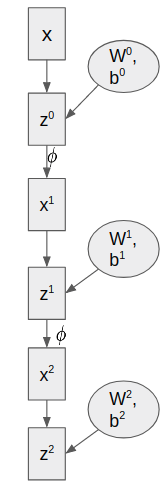
We will call $\omega$ to the set of all weights of the network. In this particular case $\omega = {W^0,b^0,W^1,b^1,W^2,b^2}$. $\phi$ is the non-linear activation function and the final mapping function is $f_\omega(x) = z^2$. We can set also a zero mean isotropic normal distribution for the prior of the weights $\omega\sim \mathcal{N}(0,\sigma_\omega^2 I)$.

For this model, the marginal likelihood equation will be:

\[p(y \mid X) = \int p(y \mid f_\omega(X), \sigma_\epsilon^2 I ) \mathcal{N}(\omega\mid 0, \sigma_\omega^2I) d\omega\]

Which as we said, this equation do not have a close form solution. Therefore, to compute the posterior of the weights of this neural network, we have to rely on e.g. Variational inference, Expectation Propagation or Monte-Carlo methods. These approaches will give us a distribution of the weights of the network $\omega$ that is close to the true posterior of the weights ($p(\omega\mid \mathcal{D}$). Once we have an approximation of the posterior we go to equation $(2)$ to obtain another approximation of the predictive posterior.

The $\mathcal{GP}$ approach

There is another path to reach the predictive posterior that does not involve finding the posterior of $f$ given the data ($p(f\mid \mathcal{D})$). This approach consists of (a) building the joint likelihood, (b) integrate out $f$ and (c) get the predictive posterior from that joint marginal distribution. This is the approach that $\mathcal{GP}$ regression follow.

First we notice that for some observed data $\mathcal{D}=(X,y)$ and some test data $(y^\star,x^\star)$, if we are given $f$, our modeling assumption $(1)$ implies that:

\[p\left(\begin{pmatrix} y \\y^\star \end{pmatrix} \mid \begin{pmatrix} X \\ x^{\star\top} \end{pmatrix}, f \right) \sim \mathcal{N}\left( \begin{pmatrix} f(X) \\f(x^{\star\top}) \end{pmatrix}, \sigma_\epsilon^2 I \right)\]

We call to this equation the train-test joint likelihood. With this joint likelihood we can try to integrate out $f$ to get the joint marginal likelihood distribution:

\[\begin{aligned} p\left(\begin{pmatrix} y \\y^\star \end{pmatrix} \mid \begin{pmatrix} X \\ x^{\star\top} \end{pmatrix} \right) &= \int p\left(\begin{pmatrix} y \\y^\star \end{pmatrix} \mid \begin{pmatrix} X \\ x^{\star\top} \end{pmatrix}, f \right) p(f\mid X) df\\ &=\int \mathcal{N}\left(\begin{pmatrix} y \\y^\star \end{pmatrix} \mid \begin{pmatrix} f(X) \\f(x^{\star\top}) \end{pmatrix}, \sigma_\epsilon^2 I \right) p(f\mid X, x^\star) df \quad (6) \end{aligned}\]

If we manage to have the joint marginal, then the predictive posterior is easy to find. If, for example, the joint marginal is gaussian, we can obtain the predictive distribution easily (see wikipedia).

Notice also that if we know the expression of eq $(6)$ we also know the expression of the marginal likelihood ($p(y\mid X)$). The predictive posterior is nothing but the joint marginal likelihood divided the marginal likelihood:

\[\require{cancel} p\left(y^\star \mid y, X, x^{\star}\right) = \frac{p\left(\begin{pmatrix} y \\y^\star \end{pmatrix} \mid \begin{pmatrix} X \\ x^{\star\top} \end{pmatrix} \right)}{p(y \mid X,\cancel{x^\star})}\]

There are two models where we can derive easily the predictive posterior distribution using the $\mathcal{GP}$ approach. The linear model and the $\mathcal{GP}$ regression.

Bayesian linear regression ($\mathcal{GP}$ approach)

The derivation of the joint marginal for the linear model is exactly similar to derivation in equation $(4)$. This leads to:

\[p\left(\begin{pmatrix} y \\y^\star \end{pmatrix} \mid \begin{pmatrix} X \\ x^{\star\top} \end{pmatrix} \right) \sim \mathcal{N}\left( 0, \sigma_\epsilon^2 I + \sigma_w^2 \begin{pmatrix} X'X'^\top & X'x'^\star \\ x'^{\star\top} X'^\top & x'^{\star\top} x'^\star \end{pmatrix}\right)\]

With this joint marginal we can apply the wikipedia formula to obtain the predictive posterior:

\[\begin{aligned} p\left(y^\star \mid \overbrace{y,X}^{\mathcal{D}},x^\star\right) &\sim \mathcal{N}\Big(x'^{\star\top}X'^\top \left(\sigma_w^2 X'X'^\top + \sigma_\epsilon^2I\right)^{-1}y, \\ &\quad\quad\quad \sigma_\epsilon^2 + x'^{\star\top}x'^{\star} - \\ &\quad\quad\quad\quad - \sigma_w^2 x'^{\star\top}X'^\top\left( X'X'^\top + \tfrac{\sigma_\epsilon^2}{\sigma_w^2} I\right)^{-1}X'x'^\star \Big) \quad (7) \end{aligned}\]

Believe it or not, this equation is equivalent to equation $(5)$! It is the same mean and covariance matrices! To show this we just have to apply the matrix inversion lemma carefully. (See also previous blog post)

$\mathcal{GP}$ Regression ($\mathcal{GP}$ approach)

We can of course retrieve the $\mathcal{GP}$ regression solution using the $\mathcal{GP}$ approach. For $\mathcal{GP}$s, we will set a extrange prior over $f$ ($p(f\mid X,x^\star$)). This prior says that any finite collection of $f(x_1),…,f(x_k)$ values is multivariate-normally distributed. The most common $\mathcal{GP}$ regression approach set the mean of such normal distribution to 0 and the covariance is given by a kernel function $k(\cdot,\cdot)$:

\[p\begin{pmatrix} f(x_1)\\\vdots\\f(x_k)\end{pmatrix} \sim \mathcal{N}\left(0, \begin{pmatrix} k(x_1,x_1) & ... & k(x_1,x_k) \\ \vdots & \ddots &\vdots \\ k(x_k,x_1) & ... & k(x_k,x_k) \end{pmatrix}\right)\]

With this peculiar prior, the integral that gives the joint marginal of eq. (6) is:

\[\begin{aligned} p\left(\begin{pmatrix} y \\y^\star \end{pmatrix} \mid \begin{pmatrix} X \\ x^{\star\top} \end{pmatrix} \right) &= \int \mathcal{N}\left(\begin{pmatrix} y \\y^\star \end{pmatrix} \mid \begin{pmatrix} f(X) \\f(x^\star) \end{pmatrix}, \sigma_\epsilon^2 I \right) p(f\mid X,x^\star) df \\ &\sim \mathcal{N}\left(0, \begin{pmatrix}K_{X,X} + \sigma_\epsilon^2 I & K_{X,x^\star} \\ K_{x^\star,X} & k(x^\star,x^\star)\end{pmatrix}\right) \end{aligned}\]

With this joint marginal we can apply the wikipedia formula to obtain the predictive posterior of the $\mathcal{GP}$ regression:

\[\begin{aligned} p(y^\star \mid y,X,x^\star) &\sim \mathcal{N}\Big(K_{x^\star,X}\left(K_{XX}+\sigma_\epsilon^2I\right)^{-1}y\\ &\quad\quad \sigma_\epsilon^2 + k(x^\star,x^\star) - K_{x^\star,X}\left(K_{XX}+\sigma_\epsilon^2I\right)^{-1} K_{X,x^\star} \Big) \quad (8) \end{aligned}\]

It is really interesting to see how this equation resemple to equation $(7)$, in fact, we would have arrive to equation $(7)$ from the $\mathcal{GP}$ regression formulation using the linear kernel $k(x,x’)=\sigma_w^2 x^\top x$!!

Neural networks ($\mathcal{GP}$ approach)

As we said before, the NNGP approach of the paper can be understood as a neural network that follows the $\mathcal{GP}$ approach to compute the predictive posterior distribution. Let’s consider the Neural Network model that we have before (figure XX) ($f_\omega(x)$). In order to find the joint marginal we have to integrate out the joint likelihood of eq. $(6)$. That is:

\[p\left(\begin{pmatrix} y \\y^\star \end{pmatrix} \mid \begin{pmatrix} X \\ x^{\star\top} \end{pmatrix} \right) =\int \mathcal{N}\left(\begin{pmatrix} y \\y^\star \end{pmatrix} \mid \begin{pmatrix} f_\omega(X) \\f_\omega(x^\star) \end{pmatrix}, \sigma_\epsilon^2 I \right) \mathcal{N}(\omega \mid 0, \sigma_\omega^2 I ) d\omega \quad (9)\]

However, as we said before, we can’t apply here Bishop’s 2.3.3. trick since the relation between $\omega$ and $x$ is not linear! Therefore we are trapped in the same problem as before and we can’t continue!

So, what is the trick that apply them to continue? Notice that in principle we could use the exact same trick to compute the marginal likelihood of the standard Bayesian approach. With this marginal likelihood we could also obtain the posterior of the weights $\omega$ and then to reach the predictive posterior using also the standard Bayesian approach path.

So what is their trick? Their proof is that on the limit of infinite width of each of the layers of the Neural Network, the joint marginal likelihood (and the marginal likelihood too) are jointly normally distributed with zero mean and covariance that can be computed using a recursive formula (i.e. is a $\mathcal{GP}$). Formally they prove that, for some kernel function $k(\cdot,\cdot)$:

\[p\left(\begin{pmatrix} y \\y^\star \end{pmatrix} \mid \begin{pmatrix} X \\ x^{\star\top} \end{pmatrix} \right)\xrightarrow[N^1,...,N^L\to\infty]{d} \mathcal{N}\left(0,\begin{pmatrix}K_{X,X} & K_{X,x^\star} \\ K_{x^\star,X} & k(x^\star,x^\star)\end{pmatrix}\right)\]

This is really cool since if we have this joint normal distribution we can apply the wikipedia formula to obtain the predictive posterior as in equation $(8)$!!

So, how do they prove it? First notice that if we assume that $y,y^\star\mid X,x^\star$ is jointly normally distributed, we just have to compute the first and second order momments to obtain the parameters of that multivariate normal distribution. Actually to compute the first momment of equation $(9)$ is not that complicated. Let’s show that the distribution of equation $(9)$ has mean zero. We will use here the same prior for the weights that is used in the paper ($W^l\sim\mathcal{N}\left(0,\tfrac{\sigma_w^2}{N_l}I\right)$ and $b^l\sim b^l\sim\mathcal{N}\left(0,\sigma_b^2 I\right)$)

\[\begin{aligned} \mathbb{E}\left[\begin{pmatrix} y \\y^\star \end{pmatrix} \mid \begin{pmatrix} X \\ x^{\star\top} \end{pmatrix}\right] &= \int\int \begin{pmatrix} y \\y^\star \end{pmatrix} \mathcal{N}\left(\begin{pmatrix} y \\y^\star \end{pmatrix} \mid \begin{pmatrix} f_\omega(X) \\f_\omega(x^\star) \end{pmatrix}, \sigma_\epsilon^2 I \right) \mathcal{N}(\omega \mid 0, \sigma_\omega^2 I ) dydy^\star d\omega \\ &= \int \begin{pmatrix} f_\omega(X) \\f_\omega(x^\star) \end{pmatrix} \mathcal{N}(\omega \mid 0, \sigma_\omega^2 I ) d\omega \\ &= \int \begin{pmatrix} x^L(X)W^L+b^L \\ x^L(x^{\star\top})W^L+b^L \end{pmatrix} \mathcal{N}(W^L \mid 0, \sigma_w^2 I )\mathcal{N}(b^L \mid 0, \sigma_b^2 I ) \mathcal{N}(\omega^{1,...,L-1} \mid 0, \sigma_\omega^2 I ) dW^L db^L d\omega^{1,...,L-1} \\ &= \int \begin{pmatrix} x^L(X)\int W^L\mathcal{N}(W^L \mid 0, \sigma_w^2 I ) dW^L +\int b^L \mathcal{N}(b^L \mid 0, \sigma_b^2 I )db^L \\ x^L(x^{\star\top})\int W^L\mathcal{N}(W^L \mid 0, \sigma_w^2 I)dW^L +\int b^L \mathcal{N}(b^L \mid 0, \sigma_b^2 I ) db^L \end{pmatrix} \mathcal{N}(\omega^{1,...,L-1} \mid 0, \sigma_\omega^2 I ) d\omega^{1,...,L-1} \\ &= 0 \end{aligned}\]

In the first step we used that the first order momment of a Gaussian is its mean parameter (which in this case is $f_\omega(X),f_\omega(x^\star)$). In the second step we applied the equation that defines the last layer of our neural network. In the third step we applied the independence of the weights, in particular we used that the weights of the last layer are independent given the weights of the previous layers. The Fourth step pull in the integral to each of the vector values and uses again the independence of the weights. Finally the last step uses again that the first order moment of a multivariate normal distribution is its mean which in this case is zero.

Since the mean of the joint distribution is zero the covariance is the second order momment. Applying the same reasoning as before, we can try to compute that covariance:

\[\begin{aligned} \mathbb{E}\left[\begin{pmatrix} y \\y^\star \end{pmatrix} \begin{pmatrix} y^\top & y^\star \end{pmatrix} \mid \begin{pmatrix} X \\ x^{\star\top} \end{pmatrix}\right] &= \int\int \begin{pmatrix} y \\y^\star \end{pmatrix} \begin{pmatrix} y^\top & y^\star \end{pmatrix} \mathcal{N}\left(\begin{pmatrix} y \\y^\star \end{pmatrix} \mid \begin{pmatrix} f_\omega(X) \\f_\omega(x^\star) \end{pmatrix}, \sigma_\epsilon^2 I \right) \mathcal{N}(\omega \mid 0, \sigma_\omega^2 I ) dydy^\star d\omega \\ &= \int \sigma_\epsilon^2 I + \begin{pmatrix} f_\omega(X) \\f_\omega(x^\star) \end{pmatrix} \begin{pmatrix} f_\omega(X)^\top & f_\omega(x^\star) \end{pmatrix} \mathcal{N}(\omega \mid 0, \sigma_\omega^2 I ) d\omega \\ &= \int \begin{pmatrix} \left(x^L(X)W^L+b^L\right)\left(W^{L\top}x^{L}(X)^{\top}+b^{L\top}\right) & \left(x^L(X)W^L+b^L\right)\left(W^{L\top}x^L(x^{\star\top})^\top+b^{L\top}\right) \\ \left(x^L(x^{\star\top})W^L+b^L\right)\left(W^{L\top}x^{L}(X)^{\top}+b^{L\top}\right) & \left(x^L(x^{\star\top})W^L+b^L\right)\left(W^{L\top}x^L(x^{\star\top})^\top+b^{L\top}\right) \end{pmatrix} \mathcal{N}(\omega \mid 0, \sigma_\omega^2 I ) d\omega \\ &=\int \begin{pmatrix} \sigma_w^2x^L(X)x^{L}(X)^{\top}+\sigma_b^2 & \sigma_w^2x^L(X)x^L(x^{\star\top})^\top+\sigma_b^2 \\ \sigma_w^2 x^L(x^{\star\top})x^{L}(X)^{\top}+\sigma_b^2 & \sigma_w^2 x^L(x^{\star\top})x^L(x^{\star\top})^\top+\sigma_b^2 \end{pmatrix} \mathcal{N}(\omega^{1,...,L-1} \mid 0, \sigma_\omega^2 I ) d\omega^{1,...,L-1} \\ &= \begin{pmatrix} \sigma_w^2 \int x^L(X)x^{L}(X)^{\top}\mathcal{N}(\omega^{1,...,L-1} \mid 0, \sigma_\omega^2 I ) d\omega^{1,...,L-1} +\sigma_b^2 & \sigma_w^2\int x^L(X)x^L(x^{\star\top})^\top \mathcal{N}(\omega^{1,...,L-1} \mid 0, \sigma_\omega^2 I ) d\omega^{1,...,L-1} +\sigma_b^2 \\ \sigma_w^2 \int x^L(x^{\star\top})x^{L}(X)^{\top}\mathcal{N}(\omega^{1,...,L-1} \mid 0, \sigma_\omega^2 I ) d\omega^{1,...,L-1} +\sigma_b^2 & \sigma_w^2 \int x^L(x^{\star\top})x^L(x^{\star\top})^\top \mathcal{N}(\omega^{1,...,L-1} \mid 0, \sigma_\omega^2 I ) d\omega^{1,...,L-1} +\sigma_b^2 \end{pmatrix} \\ \end{aligned}\]

In the first step we applied that the second order moment of a multivariate Gaussian with mean $\mu$ and covariance $\Sigma$ is $\Sigma+\mu \mu^\top$. In the second step we applied the equation that defines the last layer of the Neural Network. In the third step we used that $W^L$ and $b^L$ are independent and that the second moment of $W^L$ is $\sigma_w^2 I$ and the second moment of $b^L$ is $\sigma_b^2 I$. Finally in the fourth step we pull in the integral computation to emphasize the recurrence of the covariance of the $L$ layer with the covariance of the $L-1$ layer.

Here we cannot go further since we have the non-linear activation $\phi$: $x^L(X) = \phi(z^{L-1}) = \phi(W^{L-1}x^{L-1}(X) + b^{L-1})$. However we can recognize the recurrence of section 2.2. of the paper (eq. 2). This is the same recurrence that we can find in eq 14 of Appendix C. Bearing this in mind is easy to catch up with the reasoning of the paper to be convinced that in the limit $N_1,…,N_l\to \infty$ the joint marginal likelihood of the Neural Network is Gaussian and that we can derive a method to compute recursively the covariance of that multivariate gaussian distribution. Given that the joint marginal likelihood is gaussian we can follow the $\mathcal{GP}$ approach to obtain the predictive posterior distribution.

Bonus track: $\mathcal{GP}$ Regression (standard Bayesian approach)

In the case of $\mathcal{GP}$s, the closest thing to the posterior would be to compute the posterior on the training points $X$. We can derive this using Bishop 2.3.3.

\[\begin{aligned} p(f(X) \mid X,y) &\sim \mathcal{N}\Big(\tfrac{1}{\sigma_\epsilon^2} \left(K^{-1} + \tfrac{1}{\sigma_\epsilon^2}I\right)^{-1}y \\ &\quad\quad\quad \left(K^{-1} + \tfrac{1}{\sigma_\epsilon^2}I\right)^{-1} \Big) \\ \end{aligned}\]

To compute the predictive posterior is also not that easy because we do not have an explicit model for $f$. We have to do:

\[\begin{aligned} p(y^\star \mid x^\star,X,y) &= \int p(y^\star \mid f(x^\star), \cancel{X, y,x^\star}) p(f(x^\star)\mid X,y,x^\star) df(x^\star)\\ &= \int p(y^\star \mid f(x^\star)) \int p(f(x^\star)\mid f(X),X,\cancel{y},x^\star) p(f(X)\mid X,y,\cancel{x^\star}) df(X) df(x^\star)\\ &= \int \mathcal{N(y^\star\mid f(x^\star),\sigma_\epsilon^2)}\int p(f(x^\star)\mid f(X),x^\star,X)p(f(X)\mid X,y)df(X) df(x^\star)\\ \end{aligned}\]

In the inner integral, we can compute $p(f(x^\star)\mid f(X),x^\star,X)$ using the wikipedia formula on the joint prior:

\[p\left(\begin{pmatrix}f(X) \\ f(x^\star) \end{pmatrix}\mid \begin{pmatrix}X \\ x^{\star\top}\end{pmatrix}\right)\sim \mathcal{N}\left( 0, \begin{pmatrix}K_{XX} & K_{X,x^\star} \\ K_{x^\star,X} & k(x^\star,x^\star)\end{pmatrix}\right)\]

To get:

\[p(f(x^\star)\mid f(X),x^\star,X) =??\]

Now, since relation on $f(X)$ is linear, we can apply again Bishop 2.3.3. on the inner integral to get:

\[p(f(x^\star) \mid X,y,x^\star) = ??\]

Finally we can use Bishop 2.3.3. again to obtain the predictive distribution:

\[p(y^\star \mid x^\star,X,y) = ??\]