THE MODEL AND EXPERIMENTAL SETUP

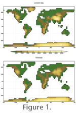
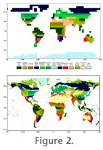
In order to perform our sensitivity experiments, we used an earth system model of intermediate complexity (EMIC) Planet Simulator (Fraedrich et al. 2005a, 2005b). The spectral atmospheric general circulation model (AGCM) PUMA-2 is the core module of the Planet Simulator. The model has a horizontal resolution of T21 (5.6° × 5.6°). Five layers represent the vertical domain using terrain-following sigma-coordinates. The atmosphere model is an advanced version (e.g., including moisture in the atmosphere) of the simple AGCM PUMA (e.g., Fraedrich et al. 1998). As compared to the first 'dry-dynamics version', the atmosphere module now includes schemes for physical processes such as radiation transfer, large-scale and convective precipitation, and cloud formation. The atmosphere model is coupled to a slab ocean and a thermodynamic sea ice model, which means that the ocean circulation is not calculated, but the heat exchange between the atmosphere and ocean is represented as a thermodynamic system. The slab ocean model uses a constant mixed layer depth of 50 m (see Lunkeit et al. 2007 for technical details). The sea ice model (based on Semtner 1976) calculates the sea ice thickness from the thermodynamic balance at the top and the bottom of the ice assuming a linear temperature gradient. In order to realistically represent the heat transport in the ocean, the models use a flux correction. It is also possible to simply force the model using prescribed climatological sea surface temperatures (SSTs) and sea ice. The thermodynamic ocean and sea ice model produces a reasonable amount of sea ice under present-day conditions (see Results), but it tends to overestimate the modern sea ice volume. It is known that the inception of sea ice in this model performs well under conditions with thin, seasonal ice (see Lunkeit et al. 2007 and references therein), but the performance for perennial ice is worse. The Planet Simulator also includes a land surface module. Amongst others, simple bucket models parameterize soil hydrology and vegetation. As compared to highly complex general circulation models, the EMIC conception of the Planet Simulator is relatively simple, but the model has a proven reliability (e.g., Fraedrich et al. 2005b; Junge et al. 2004). For a more complete description, we refer to the documentation of the Planet Simulator (Fraedrich et al. 2005a, 2005b).

For this study, we use three present-day experiments (Table 1). They all use basically the same modern boundary conditions as the highly complex AGCM ECHAM5 (e.g., Roeckner et al. 2003, 2006), but atmospheric CO₂ is set to 280 ppm (pre-industrial), 360 ppm ('normal'), and 700 ppm (enhanced), respectively. The experiments are referred to as CTRL-280, CTRL-360, and CTRL-700 in the following.

As a reference base of our CO₂-sensitivity experiments, we modelled the Late Miocene (Tortonian, 11 to 7 Ma), which we refer to as TORT-280 The boundary conditions of TORT-280 (Table 1) are based on Late Miocene simulations with the highly complex AGCM ECHAM4 coupled with a mixed-layer ocean model (Steppuhn et al. 2006; Micheels et al. 2007). The same Late Miocene configuration was used for another Tortonian sensitivity experiment with the Planet Simulator (Micheels et al. 2009). In the Miocene experiments, the solar luminosity and the orbital parameters are the same as in the present-day simulations. Orbital parameters triggered the Quaternary glacial-interglacial cycles (e.g., Petit et al. 1999), but for the Tortonian we refer to a time span of about 4 million years integrated over several orbital cycles. Due to the coarse model resolution, the Late Miocene land-sea-distribution in TORT-280 is basically the modern one (Figure 1), but it includes the Paratethys (after Popov et al. 2004). It is not possible to resolve some differences between the present-day and Miocene continent configurations. For instance, the present-day land-sea distribution represents an open Central American Isthmus because the modern land connection between North and South America is smaller than the model resolution. In the Miocene, the Panama Strait was open (e.g., Collins et al. 1996), and is represented as such in our boundary conditions. The palaeorography (Figure 1) is generally lower than present in TORT-280 (Steppuhn et al. 2006). For instance, the Tibetan Plateau reached about half of its present elevation. It should be noted that there is some debate about the palaeoelevation of Tibet (e.g., Molnar 2005, Spicer et al. 2003). Spicer et al. (2003) suggest that southern Tibet was at its present-day height over the last 15 Ma. However, the mean elevation of the Tibetan Plateau in the Late Miocene was lower-than-present (Molnar et al. 2005), which is represented in our model configuration (Figure 1). Another important characteristic in our Miocene configuration is that Greenland is lower as compared to today (Figure 1) because of the absence of glaciers (Figure 2). Also the palaeovegetation (Figure 2) refers to the Tortonian (Micheels et al. 2007). In particular, boreal forests extend far towards northern high latitudes, whereas deserts/semi-deserts and grasslands are more reduced than at present. Instead of the present-day Sahara desert, North Africa is covered by grassland to savannah vegetation in the Tortonian experiments.

The ocean is initialised using palaeo-SSTs from a previous Tortonian run (Micheels et al. 2007), and the Northern Hemisphere's sea ice is initially removed. After the initialization, we continue the model integration using the slab ocean with the present-day flux correction (Figure 3). It is commonly known that because of the open Central American Isthmus the northward ocean heat transport in the Miocene was relatively weak as compared to today (e.g., Bice et al. 2000; Steppuhn et al. 2006; Micheels et al. 2007). Later in the Pliocene, the northward ocean heat transport was stronger than today (e.g., Haywood et al. 2000a, 2000b). It is not an easy task to properly specify the ocean flux correction for a past climate situation (Steppuhn et al. 2006). With additional sensitivity experiments, it would have been possible to include different scenarios for the ocean heat transport, but this was beyond the scope of the present study because we aimed only to analyse a single factor, CO₂. Therefore, we have chosen the modern flux correction as an approximation for an intermediate state in between the relatively weak Miocene and the relatively strong Pliocene ocean heat transport. A recently published study (Tong et al. 2009) focussed on CO₂ in the Mid-Miocene using an AGCM coupled to a slab ocean model, which used a similar flux correction based on present-day SSTs and sea ice cover.

The concentration of atmospheric carbon dioxide in the Miocene is still debated and values vary from as low as 280 ppm (e.g., Pagani et al. 2005) to as high as 1000 ppm (Retallack 2001). As for the pre-industrial control experiment CTRL, atmospheric CO₂ is set to 280 ppm in the Tortonian reference simulation TORT-280. In addition, we run six experiments for which we set pCO2 to 200, 360, 460, 560, 630, and 700 ppm (Table 1). These runs are referred to as TORT-360 to TORT-700. All model experiments except TORT-200 are integrated over 200 years. The equilibrium is achieved after much less than 100 years. The last 10 years of each experiment are considered for further analysis. TORT-200 is integrated over 100 years and it is used to define a transitional experiment. From years 101 to 2100, the atmospheric CO₂ steadily increases by +1 ppm per year. This experiment is named TORT-INC and covers the range of pCO2 from 200 ppm to 2200 ppm. The maximum of 2200 ppm corresponds to a value which was realised in the Eocene (Pagani et al. 2005). We did not design a specific experiment for 1000 ppm (Retallack 2001) because, on the one hand, this value appears to be rather high for the Miocene compared to other studies (e.g., Cerling 1991; MacFadden 2005; Pagani et al. 2005). On the other hand, it is already included in TORT-INC except that the model might not be fully in equilibrium. For TORT-INC at 1000, 1500, and 2000 ppm (i.e., in years 900, 1400, and 1900), we refer to TORT-1500, TORT-1500, and TORT-2000, respectively. The setup of all our experiments is summarised in Table 1.