 CNebulaX Handbook (1.07.02, October 14th 2007)
return to the main page
José R. Torres
● CNebulaX is a freeware computer program that I have been developing through some years. It is particularly oriented to
the needs of deep sky observers, which is the
field I am most interested in. It is quite complex and you are urged to consult
this handbook to learn how to use it. The interface is very comfortable once used to it, but
it is not typical: pay thus a little
attention to the information given in this handbook. Otherwise you may ignore
the right way of operating the interface, and the program will be used
clumsily. Alternatively, you can see a short slideshow when
the program starts, informing on the basic usage.
● CNebulaX is offered to you altruistically.
I am earning nothing. It is offered to the community of amateur astronomers as
a gift, so take this into account and if you need contacting me, please be
polite and cooperative. After learning how to use CNebulaX,
people are generally satisfied and I have received quite encouraging emails. If
you like CNebulaX I will be very glad; if not, please
do not complain and just erase it. After all, you have paid nothing for it.
CNebulaX
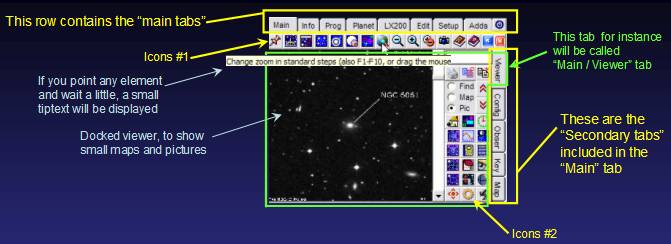
works with two windows: the MAIN MAP (always visible filling the screen) and the TOOLBOX (the tabbed area usually located at the
lower left corner of the screen, but can be hidden below the main map or moved
to other screen locations). There are many other secondary windows. The VIEWER for instance is a floating window to show pictures and secondary maps,
and the OBSERVING
PLAN VIEWER shows special plots and pictures of
the objects within the observing list you are creating, or editing. The toolbox
is the core of the program and includes all control components in sorted tabs.
The toolbox
structure mimics a pull down menu (see the
picture): top
tabs for main entries,
right
tabs for associated items to each main tab,
and sometimes bottom
tabs for sub-options associated to a given the
secondary tab. This yields more room and a more informative layout: you can
view all the information and perform operations in a few clicks. Text tips are
displayed if you put the mouse on the element you want to know and wait for a
while. The program is simple to use, but you have to learn small tricks and
some protocols. Here you will find a basic knowledge on the use of the program
and some operations not so obvious. Remember that there is also a slideshow
available when the program starts. I have sorted the operations to allow an
easier location of the task you may want to do:
 ● Installation and first run: CNebulaX
configuration
● Installation and first run: CNebulaX
configuration
● Running the program: the TOOLBOX
● The VIEWER and the information cards
● Changing the magnification
● Finding objects: the JUMP combo box and Quick DSO picker
● Rotate/Flip the map and horizontal modes
● Overlaying reference circles, CCD frames
and eyepieces
● Planetarium, ephemeredes and complementary information
● Navigating through the Sky
● Print / copy / paste text, maps and pictures
● Making observation lists (or programs)
● Making notes
● Comets, asteroids and planets. Plotting orbital trails
● The CNebulaX main library (Reference)
● Control of LX200 classic telescopes
● Identification of deep sky objects: matching maps and
pictures
 • BEFORE STARTING: Update CNebulaX to the latest release, and install all the
supplementary databases and updates. Some features (special orbits, custom
printouts, slideshow help) are only available in the
latest release. Note that there can be discrepancies between the handbook and
the CNebulaX version you are using: they may be not
synchronised and I am always making small improvements.
• BEFORE STARTING: Update CNebulaX to the latest release, and install all the
supplementary databases and updates. Some features (special orbits, custom
printouts, slideshow help) are only available in the
latest release. Note that there can be discrepancies between the handbook and
the CNebulaX version you are using: they may be not
synchronised and I am always making small improvements.
• SOME LINKS:
● CNebulaX main page
● CNebulaX download page
Setup files and instructions for
making a basic installation
● CNebulaX complements page
Extra databases to expand the basic
installation
Latest compiled EXE file
● CNebulaX latest handbook
Latest modified handbook
● CNebulaX FAQ
● Root webpage
● Contact by email
VERY IMPORTANT: Entering information in the text
boxes
In
CNebulaX there is no "Apply" or
"Proceed" buttons to apply changes: the ENTER key does it instead. You
will see lots of small text boxes to introduce information. After modifying the content of any text
box, press the ENTER key to
apply the changes you have done. Also, there is a special combo box
(i.e., text box + dropdown list) called the JUMP combo box, which allows
entering objects names, planets or constellation codes. Thus, for instance, for
centring the main map the globular cluster Messier 13, just type "M
13" (without quotations) in the jump combo box, and press ENTER.
To top
 Download the installation file and unzip the content in whatever temporary
place. Double click the SETUP.EXE to run the
application. Follow the instructions given. Install the program close to the
root folder (e.g., C:\INDEX).
Download the installation file and unzip the content in whatever temporary
place. Double click the SETUP.EXE to run the
application. Follow the instructions given. Install the program close to the
root folder (e.g., C:\INDEX).
The
first run will require that you specify the working folders. There are five
folders to specify. The first two are essential for running the program.
Root CNebulaX folder – Corresponds to the installation folder that you have selected during
the installation process. All the program files are stored within this folder.
Star database
– This entry allows changing the main star database. I have several databases
coming from earlier stages in the development. I conserve this entry for
maintenance reasons, so do not worry for this entry, and set the same folder as
in the former entry (RootCNebulaX folder).
When
the program is installed, you only have to verify that these two entries are
right. The remaining entries are optional and correspond to image folders. At
this point, don't worry for them, and ignore warning messages. CNebulaX is prepared to show pictures in the viewer as you
navigate through the maps. Probably you will decide to use them in the future,
but not in the first run. There are three categories of image folders:
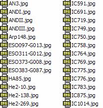
IMAGEDB - root main image folder,
which contains several subfolders, one for each object class (OPNCL, GLOCL, GALXY,
CL+NB, PLNNB, BRTNB, etc). A given object file should be stored according
to its class in the respective subfolder (e.g., "M 97" within PLNNB, "M 31" within GALXY,
etc)
USERDB - User database folder. It is a special folder that can contain unclassified graphic files
(without subfolders). It is not recommended to use this folder to store all
images since it would slow down the program. However, it can be used for
storing a "small" collection (i.e., less than one thousand images)
DSS - Digital Sky Survey files. If the NGC/IC project has been downloaded
for offline browsing and the location of the DSS
subfolder properly specified in the Setup/Config/Files
tab, the program will display the pictures.
 Since the NGC/IC project represents a thorough revision of NGC and IC
objects. I have given to DSS higher hierarchy for
being displayed. So, the order is: (1) DSS, (2) IMAGEDB, and (3) USERDB. The
displayed image corresponds to the first file found following this sequence.
However, you can easily select other alternative images (if exist), since there
is an icon in the toolbox (the small camera in the first row of the main/viewer
tab -see the toolbox picture-) to select them.
Since the NGC/IC project represents a thorough revision of NGC and IC
objects. I have given to DSS higher hierarchy for
being displayed. So, the order is: (1) DSS, (2) IMAGEDB, and (3) USERDB. The
displayed image corresponds to the first file found following this sequence.
However, you can easily select other alternative images (if exist), since there
is an icon in the toolbox (the small camera in the first row of the main/viewer
tab -see the toolbox picture-) to select them.
The
program recognizes other special folders/subfolders (i.e., PGC
and specific folders for different object classes: PLNNB,
GLOCL,...) existing in my
personal release. CNebulaX is prepared to manage this
structure of image folders. However, I cannot provide images because in some
cases have been purchased and/or are subjected to copyright restrictions.
Moreover, the size is immense: I have near 200,000 pictures filling 2 Gb. I would recommend you to
download at least the NGC/IC project files with an off-line browser; it is an
excellent starting point. Image file names must coincide with the CNebulaX names without spaces, in JPG or GIF formats (e.g.,
M45.JPG, NGC1528.GIF).
There is more information on this below.
When you click the
proceed button, the program will close. Don't worry; this is normal, since a
new INI file is being created. So when it closes,
just reload CNebulaX again and the new specifications
will be applied.
To top
Go
to the folder you selected for the installation (RootCNebulaXFolder),
and right-click in CNebulaX.EXE
file. Then select "create shortcut"
in the pop-up menu you will see. Right click on the shortcut icon, and select "properties". Be sure you see in
the "Start in" entry the folder location where CNebulaX.EXE
was stored; if not, add it. Finally, move the shortcut icon to whatever
place in your PC (the desktop, start menu, etc).
To top
• ARRANGEMENT: The toolbox includes
several collections of sorted tabs. The eight "MAIN" tabs are placed
in the upper area of the toolbox (see the picture). The secondary tabs are
vertically arranged in the right area within each Main Menu tab, and lead to
specific operations. This arrangement is equivalent to the classical menus in
many computer programs, but in my opinion, with the tabs arrangement we get a
more practical and informative layout. It was also the most compact way I could
find of fitting the picture viewer together with the controllers, and once used
to it, it is really comfortable.
USE OF TEXT BOXES - There are lots of
small text boxes to enter information. After modifying the content of any
text box, press the ENTER key to apply the changes you have
done. There is no button to apply
changes: they are applied pressing ENTER. (Repeated
message to emphasize the importance)
The general
arrangement of the toolbox (it can change from one release to another) is as
follows:
MAIN
TABS: they are located in the upper border
of the toolbox, and consist of the following tabs: (1) Main,
(2) Info, (3) Prog, (4) Planet,
(5) LX200, (6) Edit,
(7) Setup, (8) Adds. Let's see the general purpose of the main and
secondary tabs:
|
(1) Main: it includes the most practical controllers associated
to the main map.
Viewer (most used
tab) - it frames the docked viewer and the most usual controllers.
Config - configuration of the main map (specifications to setup
the map).
Observ - notes of the visual appearance of DSOs (only NGC and
IC at the moment).
Key - legend with the
symbols used in the main map.
Map - DSOs labels and
information associated to the pointer (mouse).
(2) Info: information for the current object and ephemeredes for
planning its observation.
Data - Data for the
current object (position, classification, charts, rise, etc).
Notes - Personal
notebook (for your own annotations at the telescope, comments, etc).
Day - Plot showing the
daily trend (height vs. time) for the Sun, Moon and current object.
Month - Month trend
(rise, transit and set) for Sun, Moon and the current object.
Years - Annual plot
(rise, transit and set) for current object, and twilights.
Find - Finder view of
the current object with independent inversions.
(3) Prog: construction/edition of observation programs (=make/edit
observing lists).
Database - Select the
databases to be used in the cross searches.
Cross search - Specify the
conditions to fulfil in the cross search, and proceed to it.
Manage output - Review, edit and
save the list of objects found in the cross search.
(4) Planet: Sky planetarium
and ephemeredes for comets, asteroids and main planets
Sky - planetarium
view for the current object, planets, Sun and Moon. It also allows selecting
instants in the current Julian date and edit Earth views
Comet - select and map the currently visible comets
Ast - select and map
the currently visible asteroids
Planet - get accurate information of the main
planets and select the orbit theory
Model - default values for the simulation of
asteroids and comets
(5) LX200: Control of
LX200 classic telescope (at the moment, it only controls my main telescope)
Telescope - connection,
speed, motions, slews, synchronization and information
Serial port setup - setup of the
serial port
Port monitor - it shows the
data send to or received from the RS232C port
(6) Edit: Send
information to the printer or clipboard (maps), and configure the associated
options.
(7) Setup: Configure CNebulaX, your telescope, accessories and observing
place.
Configuration - telescope,
eyepieces, limiting magnitude and screen features.
Date/Time - change the
geographical situation, date, time and time offset.
Custom colours - change the
colour set (it is saved in the INI file).
(8) Adds: Some operations
not classified in the previous tabs or under development
Image - overlay maps on
pictures to identify objects, and edit undocked images
Binary - calculate ephemeredes
for visual binary stars (orbital pairs).
Ephem - calculate
general ephemeredes (still growing)
Overlay - get an external
file with header information to overlay it
System - system
maintenance (hidden features in public releases)
|
Secondary tabs

This tab arrangement corresponds to
a recent compiled EXE file, but it is not the last one
If you detect changes, you can be
using either an older or a newer version. Anyway, the essential points will
be equally valid.
The Main/Viewer tab includes
the most common controllers and the docked viewer. It is the one shown when
the program starts, and auto-retrieves the focus in most operations because its utility for performing general operations.
|
For further sections, it will be followed this
convention: a given combination MainTab-SecondaryTab
will be expressed as Main/Secondary, for instance: "Prog/Cross search" or "Info/Notes".
The main frame shown when the program is activated is the "Main/Viewer"
tab.
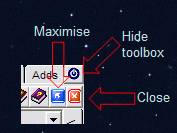
 • SWITCH BETWEEN NORMAL/MAXIMISED VIEW: The
usual way is running CNebulaX maximised, filling the
whole screen. However, a more compact view can be sometimes of interest. This
can be accessed from the maximise-minimise
icon in the toolbox (blue icon at the right of the "Adds" tab, in
the Main/Viewer tab). To return to the maximised view, click on the same icon
again. The program is never minimised: it can only work in normal or maximised
modes. The way of changing the window modes is somewhat awkward. However, you
should avoid setting the program in normal mode: it is not recommended.
• SWITCH BETWEEN NORMAL/MAXIMISED VIEW: The
usual way is running CNebulaX maximised, filling the
whole screen. However, a more compact view can be sometimes of interest. This
can be accessed from the maximise-minimise
icon in the toolbox (blue icon at the right of the "Adds" tab, in
the Main/Viewer tab). To return to the maximised view, click on the same icon
again. The program is never minimised: it can only work in normal or maximised
modes. The way of changing the window modes is somewhat awkward. However, you
should avoid setting the program in normal mode: it is not recommended.
• CLOSING CNebulaX
AND SAVING THE INI FILE: There are two ways of
closing the program:
(1) Close icon in
the Toolbox
(2) Close icon in the Main Map
Both
close icons terminate the program showing the SAVE INI
dialog (it allows saving the configuration at your will). If you accept
saving the configuration and have loaded or created an observing program, or
modified the list of eyepieces and focal modifiers, the close dialog also saves
them. There are extra buttons to save specifically the INI
file (Setup/Configuration tab, "Save INI"
button) and the observation list or program (Prog/Manage
Output tab, "Save" button). Only some features are stored in the INI file: the remaining ones are reset to the default
values in the next loading, since after having used the program thoroughly, I
found it more convenient.
• SHOW / HIDE THE TOOLBOX:
• MOVE THE TOOLBOX: As
mentioned, the toolbox is situated in the lower left corner of the screen.
However, sometimes you'd rather put it in another place. Moving it is easy:
just double click on any of the upper tab captions of the toolbox (i.e., the
main tabs), holding the button after the second click. Then, without
releasing the button, drag the toolbox to the place you wish. Finally, release the
mouse button.
To top

 • DISPLAYING THE DATA FOR THE OBJECTS IN THE MAP (picture, map or
finder map) Right click with the mouse on the symbol of any
object plotted within the main map. This will display a card with the data of
the nearest object to the clicked point.
• DISPLAYING THE DATA FOR THE OBJECTS IN THE MAP (picture, map or
finder map) Right click with the mouse on the symbol of any
object plotted within the main map. This will display a card with the data of
the nearest object to the clicked point.
 As you see, the basic information
will be shown in a small card with the essential data:
As you see, the basic information
will be shown in a small card with the essential data:
 • Left
click on
the information card to close it
• Left
click on
the information card to close it
• Right
click on the information card for a pop-up menu
By
default, the information card system works on deep sky objects planets and
double stars. If you want to apply it to stars, then you should click on the pointer
mode icon (at the left of the clock icon in the toolbox).
For most NGC
and some IC objects, the Main/Obs tab shows
information about the telescopic appearance. This information has been
collected in the net and I have organised it to be accessible in the
navigation. If you can get observational info of good quality and you agree
sharing it in this project, send me an ASCII file and I will compile it for the
inclusion. My intention is compile a huge database with observations. Alternatively, you can also consult the
CNebulaX reference , where more observational
data is available.
 More
information is given in the Info tab and the associated sub-tabs. The basic
data sorted by fields are given in the Info/Data tab. The remaining tabs allow
taking notes (and see them), display the basic ephemeredes for the current
object (day, month and year views), and an independent map that can be fitted
to your finder features. All these plots will be explained in a specific
section, below.
More
information is given in the Info tab and the associated sub-tabs. The basic
data sorted by fields are given in the Info/Data tab. The remaining tabs allow
taking notes (and see them), display the basic ephemeredes for the current
object (day, month and year views), and an independent map that can be fitted
to your finder features. All these plots will be explained in a specific
section, below.
The information of the information
cards can be altered from the Main/Config tab to full
cards or short cards ["Full cards" check box], and with or without
rise/transit/set data ["Rise/Set" check box].
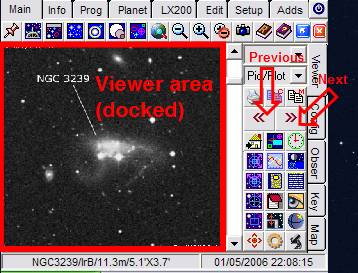
• NEXT / PREVIOUS NEAR OBJECT: Click
on the buttons with the symbols [<<] and [>>] to jump to the
previous and next near object, respectively. You can cycle through the objects
situated at a small distance of the clicked point with those buttons. Each time
you right click on a new object, the exploration environment is also refreshed
for the new object. It is a very comfortable system even to explore very
crowded areas.

• THE VIEWER: It
is used to display pictures or small maps of the deep sky objects we are
selecting. Thus, if the viewer is enabled, each time you right clicking on
any object plotted in the main map, the viewer will show:
 (1) its picture
(2) a small map centred on it
(3) a finder view, or
(4) its basic data
This is whatever the choice you have
selected in the viewer mode combo box (Main/Viewer tab).
The viewer can be disabled from the same combo
box. In addition, there are two viewer modes:
(1) In the docked mode (default),
the viewer is fitted within the toolbox (Main/Viewer tab)
(2) If the viewer is in the undocked
mode, it is shown in an independent window
If
the object is shown as a picture, left clicking on the picture will undock the
viewer. If you then click again in the undocked viewer window, it will be
docked again within the toolbox.
• Left click on the main map
pressing CTRL = it will show the magnified area in
the viewer.
• DISPLAYING PICTURES IN THE VIEWER: CNebulaX is designed to show
pictures, but I cannot provide any image collection. If you download images
from the net, or buy from somebody else an image CD, NebulaX
would be able to display them.
 My
release for personal use includes a large image database including about
150,000 images of deep sky objects from POSS and
other sources (virtually, one picture for any displayed object in a
mean-expanded basic installation). Each time I click on an object, the viewer
plots it. For doing it, however, the image file should follow certain rules for
the name, and be located in a folder named as the object type in NebulaX. For instance, M 76 will be displayed if a file
called "M76.JPG" exists on a directory
"PLNNB" under the [Imagedb]
folder specified in Setup/files. If you have downloaded the NGC/IC project site
with the file structure unaltered, the DSS folder can
also be specified. I have completed all objects of NGC and IC starting from the
NGC/IC collection.
My
release for personal use includes a large image database including about
150,000 images of deep sky objects from POSS and
other sources (virtually, one picture for any displayed object in a
mean-expanded basic installation). Each time I click on an object, the viewer
plots it. For doing it, however, the image file should follow certain rules for
the name, and be located in a folder named as the object type in NebulaX. For instance, M 76 will be displayed if a file
called "M76.JPG" exists on a directory
"PLNNB" under the [Imagedb]
folder specified in Setup/files. If you have downloaded the NGC/IC project site
with the file structure unaltered, the DSS folder can
also be specified. I have completed all objects of NGC and IC starting from the
NGC/IC collection.
If pictures are not available, the
viewer in the photo mode will just plot normal or finder maps (this is,
simulating the telrad circles), but if the object is
a double star, it simulates it at scale (in the undocked mode), and if it is a
variable star, overlaying the magnitudes of neighbouring stars. If you prefer
reducing the functionality of the viewer in order to gain speed, just select
the "Data only" option button within the main tab of the toolbox, or
disable it. You can change the displayed mode at any moment from the viewer
mode combo box.
CNebulaX can display
pictures, provided some cautions are kept:
● The allowed formats are GIF or JPG
● Each file name should coincide with the
respective object name in the database without spaces: A file for "PK 164+31.1" could be "PK164+31.1.JPG",
and "NGC7331.JPG" is a graphic file for NGC
7331
● The files should be properly stored in
the folders indicated in Setup/Config/Files tab
 How do the image folders work?
- Three
categories of image folders are established:
How do the image folders work?
- Three
categories of image folders are established:
USERDB (the name and location are arbitrary)
- the user image folder. It is a special folder that can contain unclassified
graphic files (without subfolders). It is not recommended to use this folder to
store all images since it would slow down the program. However, it can be used
for storing a "small" collection (i.e., less than one thousand). By
default CNebulaX install a folder called [ImageDB\User]. In USERDB you can
specify a second folder with the same functionality than the [ImageDB\User] folder.
IMAGEDB - the
root main image folder, which contains several subfolders, one for each object
class (OPNCL, GLOCL, GALXY, CL+NB, PLNNB,
BRTNB, etc, see the picture). A given object file
should be stored according to its class in the respective subfolder (e.g.,
"M 97" within PLNNB, "M 31"
within GALXY, etc). As just mentioned, IMAGEDB also contain the special folder called
"User" for non classified images, similarly to USERDB.
DSS - The Digital Sky Survey files. If the
NGC/IC project has been downloaded for offline browsing and the location of the
DSS subfolder properly specified in the Setup/Config/Files tab, the program will display the pictures.
 Since the NGC/IC project represents a thorough revision of NGC and IC
objects. I have given to DSS higher hierarchy for
being displayed. So, the order is: (1) DSS, (2) IMAGEDB, and (3) USERDB. The displayed
image corresponds to the first file found following this sequence. There are
other special folders/subfolders (i.e., PGC).
Since the NGC/IC project represents a thorough revision of NGC and IC
objects. I have given to DSS higher hierarchy for
being displayed. So, the order is: (1) DSS, (2) IMAGEDB, and (3) USERDB. The displayed
image corresponds to the first file found following this sequence. There are
other special folders/subfolders (i.e., PGC).
There is an icon
with a photo machine in the Main/Viewer tab. From there, you can launch a
pop-up menu to select a second view of the object (if it there are images in
more than one folder), or load any image file in the viewer.
• DOUBLE STARS: Double stars in the main map are
displayed as in Herald-Bobroff's Astroatlas,
that is, at scale (in NebulaX the scale is, however,
logarithmic to extend the plotting range). The double stars are labelled with a
separation (number 0-9) / magnitude (character A-E) code. The number indicates
the difference in brightness between the main and the secondary component, and
the character, a separation class code, being A a very close double stars and E a very sparse double. A
very good double star, let's say 6.5 and 6.8 components separated 3.5",
will appear labelled in the map as "0C".
The viewer, if is undocked, plots the stars at
scale at would be seen from the viewing distance you have specified in the
Setup/Configuration tab. If it is in the docked mode, the image will be slightly
smaller
To top
 There
are several ways to get this, being the most comfortable by dragging the mouse
on the main map. Try it, it is really handy.
There
are several ways to get this, being the most comfortable by dragging the mouse
on the main map. Try it, it is really handy.
Just
click on the centre of the region you want magnify and drag the map downwards
if you want to expand it, or upwards if you want to get a wider view. The zoom
caption will show you the target magnification. When you have reached the value
you want to set, just release the mouse and the main map will be re-plotted
with the new values.
• ZOOM IN =
drag the mouse downwards on the star chart, and
release it. The current magnification is displayed in the caption of the zoom
box you will see.
• ZOOM OUT= drag the mouse upwards and release it.
• CHANGE IN STANDARD STEPS:
F1 (greater) - F10 (smaller magnification). There is also an icon in the
Main/Viewer tab (symbol: Earth with a magnifier), which displays a pop-up menu
for the selection of the most usual magnifications.
• SLIDER: Alternatively, you can
use the slider within the Main/Config tab of the
toolbox
• ZOOM TEXT BOX: Just above the slider, there is a text box where you can specify the
degrees you want to apply (vertical scale). As usual, press ENTER to apply
changes.
• SWAP EXPLORATION / DETAIL ZOOMS:
The two zoom values (exploring/examining) specified in the Main/Config tab can be swapped by clicking certain icon in the
Main tab, with two overlaid (red and blue) magnifiers.
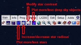
 The most important map configuration
controls govern the number, size and contrast of stars, and the number of deep
sky objects, which are also accessible also from the Main/Viewer tab:
The most important map configuration
controls govern the number, size and contrast of stars, and the number of deep
sky objects, which are also accessible also from the Main/Viewer tab:
●
Mag:
limiting magnitude in the main map. Once modified, it is maintained whereas is
unchanged. When the zoom is changed, the limiting magnitude is autocalculated again and the former value set the user, overwritten.
●
m-offset: magnitude
offset to be added to the automagnitude value. If you
want less stars, put a negative value (e.g., ‑0.5) and if your screen is larger
and you want more stars, put a positive value (e.g,
+0.5)
●
r-offset: star size offset
that make the stars appearing larger. Introduce a value larger than zero (e.g.,
+0.5) to enlarge stars, and a negative one (e.g, ‑0.5) to make
them smaller
●
Level: contrast
value, that make the progression in bright soft or more sudden (a value form 1
to 10). A mid value (5) gave a nearly linear increment in star radius.
 The
Main/Config tab includes other options to customise
the maps. There is a set of check boxes (lower left area). Full screen removes the main map caption. Planets activates/desactivates the planets, Sun and Moon. Eq.grid switches the grid of equatorial coordinates. Zenith activates the Earth view (pseudo horizontal mode). Labels removes the labels for identify
the objects in the main map. Mag plots/removes
the magnitude for stars. Full
cards adds extra information (notes) in the information cards. Rise/set adds to the information card
of the active object the instants of rise, transit and set. Varst, Dblst and DSO adds/removes
variable stars, double stars and deep sky objects, respectively. Restrict DSO filters the deep sky
objects to only plots Messiers, NGCs
and ICs. MWay adds/removes the Milky Way. HLeda labels forces to label HyperLEDA galaxies (provided they are plotted), instead of
only labelling them at a high magnifications. Finally, Horiz plots/removes the horizon line. All these switches allow a
considerable degree of customisation.
The
Main/Config tab includes other options to customise
the maps. There is a set of check boxes (lower left area). Full screen removes the main map caption. Planets activates/desactivates the planets, Sun and Moon. Eq.grid switches the grid of equatorial coordinates. Zenith activates the Earth view (pseudo horizontal mode). Labels removes the labels for identify
the objects in the main map. Mag plots/removes
the magnitude for stars. Full
cards adds extra information (notes) in the information cards. Rise/set adds to the information card
of the active object the instants of rise, transit and set. Varst, Dblst and DSO adds/removes
variable stars, double stars and deep sky objects, respectively. Restrict DSO filters the deep sky
objects to only plots Messiers, NGCs
and ICs. MWay adds/removes the Milky Way. HLeda labels forces to label HyperLEDA galaxies (provided they are plotted), instead of
only labelling them at a high magnifications. Finally, Horiz plots/removes the horizon line. All these switches allow a
considerable degree of customisation.
 The colours of most plotted objects can be changed
from the Setup/Custom colours tab. The upper option buttons allows returning to
some default colours in single click. The current colour configuration is saved
in the INI file, but custom colours are overwritten
with default colours if you return to them with the upper option buttons.
The colours of most plotted objects can be changed
from the Setup/Custom colours tab. The upper option buttons allows returning to
some default colours in single click. The current colour configuration is saved
in the INI file, but custom colours are overwritten
with default colours if you return to them with the upper option buttons.
 Finally,
the Main/Map tab includes some other controls. The DSO Labels frame allows
selecting the mode in which the stars and deep sky objects will be labelled in
the main map. By default, the labels are the name for deep sky objects and
variable stars, and a magnitude/distance code for double stars. These values
can be replaced by a summary line, magnitude, notes, and some others. The map
font can be selected from the button just below, and the check box besides it
can set the information cards background to transparent. The check box [do not
use caption] displays the pointer information on the main map (lower right
area) instead of in its caption.
Finally,
the Main/Map tab includes some other controls. The DSO Labels frame allows
selecting the mode in which the stars and deep sky objects will be labelled in
the main map. By default, the labels are the name for deep sky objects and
variable stars, and a magnitude/distance code for double stars. These values
can be replaced by a summary line, magnitude, notes, and some others. The map
font can be selected from the button just below, and the check box besides it
can set the information cards background to transparent. The check box [do not
use caption] displays the pointer information on the main map (lower right
area) instead of in its caption.
REVISED UP TO
HERE
To top
Get
the Main/Viewer
tab of
toolbox, and look for an empty combo box (=text+list
box) in the upper-right area. This is the Jump combo box. There are two ways of using this control,
which is the CNebulaX generic search facility:
 MODE
1 -
Enter straightforwardly the object name in the text area of the combo box. After typing the name, do not
forget pressing the ENTER key to jump to the object.
MODE
1 -
Enter straightforwardly the object name in the text area of the combo box. After typing the name, do not
forget pressing the ENTER key to jump to the object.
MODE 2
- Click the right button to deploy the hidden associated list. You will see a
number of predefined targets (the Planets, Sun and Moon, Comets, Asteroids, Herschel'400 or Messier lists, Constellations, and others).
You can click on the items in the list to select the target you wish. There are
three kind of targets: (1) Direct targets (Sun,
Moon and planets) that once clicked, move the map to them, (2) Comets and asteroids, that should be selected
specifically from the Planet/Com or Planet/Ast tabs, (3) Lists within the Main Reference (Messiers, Herschel 400, Main stars, etc). This kind of
entry activates the main library and the final object should be selected from
lists. Once selected an entry in the main reference list, just click on the
purple book icon with and "R" to display the list again and make a new
choice.
The reference library also includes dozens of
tables that can be clicked to jump to deep sky objects. The use of this
facility will be seen later.
Alternatively to Mode-1, you can also use the "Center
the map in" box in the Main/Config tab
 • Common
objects: If you want to center let's say
M22, type "M22" and ENTER, and that's it. NGCs
do not require any prefix ("N" or "NGC"), just the number.
If the number is 1-110, it is interpreted as belonging to a Messier object, so
if you want to center NGC 80 type "N 80",
"NGC 80", otherwise you will jump to M 80. There are some other tents
of abbreviations, A for Abell, I for IC, etc.
• Common
objects: If you want to center let's say
M22, type "M22" and ENTER, and that's it. NGCs
do not require any prefix ("N" or "NGC"), just the number.
If the number is 1-110, it is interpreted as belonging to a Messier object, so
if you want to center NGC 80 type "N 80",
"NGC 80", otherwise you will jump to M 80. There are some other tents
of abbreviations, A for Abell, I for IC, etc.
• Constellations If you select "Constellations"
in the combo box entry, a list of constellation will be displayed to select
which one you want to see. Click on the one you prefer and the main map will be centered on it without altering the main
map magnification. Alternatively, you can type directly in the combo box
the constellation code (e.g., Aql, And, Ori, etc). In that case, the constellation will be centered and the magnification changed to get a full
view.
• Planets and others: You can also type a planet name (Mars), Sun or Moon to jump to it
(+ENTER, as usually). Minor planets and comets cannot be entered directly, and
should be selected from the Planet/Ast and Planet/Com
tabs, since they require being first loaded by the system.
 • Equatorial coordinates: You
can also input the equatorial coordinates in the "R.A."
and "DEC." text boxes. Pressing J (jump) with the map activated shows
the jump facility as well. The coordinates are not accessible from the jump
combo box.
• Equatorial coordinates: You
can also input the equatorial coordinates in the "R.A."
and "DEC." text boxes. Pressing J (jump) with the map activated shows
the jump facility as well. The coordinates are not accessible from the jump
combo box.
• Reference library - You can also use
the reference library facility (icon with a book with and R in the cover) to
select your target and jump examining the tabulated data. It keeps the position
of the last clicked target for an easier navigation: click on the book again
and make a new selection when you wish.
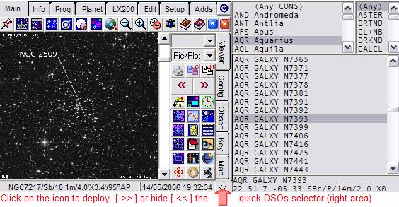
 Quick DSOs picker
This
facility works directly on the "general" database, and allows
building quick lists to examine the main objects (data and pictures) by constellations
and/or object type. It is activated from the small icon raised in the image
below, which deploys [>>] or hides [<<] two interlinked lists:
constellations and object class. These lists can be used to see the deep sky
objects fulfilling the selection. If you have linked images to CNebulaX, single clicking on the found DSOs (or moving on the list
with the arrows keys) will show a picture in the viewer and some extra data. Double click on the list will centre
the map in the selected object, and will set it as the active one.
Quick DSOs picker is a new feature included in the 1.05.65rs
To top
 • PANNING IN THE MAP:
(1)
Left click with
the mouse in the point you want to center in the main
map = center the map at the pointed coordinates.
(2)
Alternatively, the arrow keys also
move the map to the neighbouring areas.
• ROTATE THE MAP:
(1) Rotation textbox (Main/Config tab): write the
rotation angle and press ENTER.
(2) Rotate map icon (Main/Viewer
tab): Maps can also be rotated graphically with one of the icons in the Main/Config tab. Once activated the rotation tool, a line will
be displayed indicating the tentative direction of the top of the map, which
can be changed with the mouse. Once defined the new orientation, click on the
map to apply it.
• FLIP THE MAP (INVERSIONS):
 SINGLE INVERSION:
(1) If your telescope
inverts the image once (prism), and you want the maps left-to-right inverted,
mark the FLIP-Horiz checkbox.
The maps can also mirrored up-to-down by clicking FLIP-Vertical
checkbox in the Main/Config
tab.
(2) Alternatively: activate the horizontal flip
/ vertical flip icon (each of them will be highlighted if
it has been activated).
DOUBLE
INVERSION: If your telescope inverts the image
twice (astronomical telescopes), set rotation angle to 180.
Alternatively, activate both flip icons.
Naturally, you can alter these values with
the ROTATE MAP facility to match exactly the telescope appearance.
 • HORIZONTAL MODES (true- and pseudo- horizontal modes):
CNebulaX includes two
horizontal modes (or earth views):
 (1) True horizontal mode - it is accessible from the Planet/Sky
tab, but it is not applied to conventional maps since it makes them slower to
be plotted. The true horizontal mode is only applied in the two kinds of sky
plots accessible from the Planet/Sky tab.
(1) True horizontal mode - it is accessible from the Planet/Sky
tab, but it is not applied to conventional maps since it makes them slower to
be plotted. The true horizontal mode is only applied in the two kinds of sky
plots accessible from the Planet/Sky tab.
(2)
Pseudo-horizontal mode - in practice, it
allows plotting maps quite comparable true horizontal maps for zooms <30º,
but it is faster. It just rotates the chart to point its centre oriented
towards the zenith. For telescopic or binocular views, this strategy is far
more preferable and completely equivalent to the former horizontal mode. For
activating it:
(2a) Zenith
check box (Main/Config
tab): if checked, the top of the map will be always pointed to the zenith. The
default way (unchecked) allows rotating the map freely.
 (2b) There is also an icon in the Main/Viewer tab to activate the horizontal mode.
• RETURN TO THE STANDARD MODE: to return the map
to the standard mode (unrotated, unflipped
and with the north at the top), you can unmark one by one the icons you have
previously clicked to get the inversions/flips, but you can do it in a single
operation by clicking the "remove flips & rotations" button with
a house (Main/Viewer tab).
To top
 • OVERLAY REFERENCE CIRCLES: By default, a 1 degree black circle is drawn at the map center, surrounded by a 5 degree red circle simulating the finder view. The
dimensions of both circles can be changed to whatever value from the text box
you will see in the Main/Config tab (leave the box
empty to hide the circles). You can also specify more circles separating them
by [;] (e.g., "1;2;4;7"). The first circle
in the list is the "Main Circle", which will be filled. Do not use this facility to set
your eyepiece field, since there is an easier and handier way to overlay
eyepieces fields (see
below). Reference circle are just that: references that make understanding the
map scale easier.
• OVERLAY REFERENCE CIRCLES: By default, a 1 degree black circle is drawn at the map center, surrounded by a 5 degree red circle simulating the finder view. The
dimensions of both circles can be changed to whatever value from the text box
you will see in the Main/Config tab (leave the box
empty to hide the circles). You can also specify more circles separating them
by [;] (e.g., "1;2;4;7"). The first circle
in the list is the "Main Circle", which will be filled. Do not use this facility to set
your eyepiece field, since there is an easier and handier way to overlay
eyepieces fields (see
below). Reference circle are just that: references that make understanding the
map scale easier.
The tip in the Main Circle is always pointed
to the zenith and allows referring the maps to the actual orientation in
the sky.
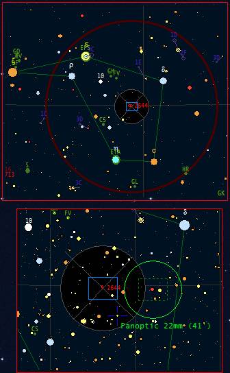
• OVERLAY EYEPIECE
FIELDS:
 Left click with the mouse pressing
SHIFT.
It displays overlaid the field seen through the current eyepiece. The eyepiece
class and focal length can be changed from the Setup/Configuration tab in the
toolbox (click on the lower label to activate this). The default eyepiece is
one of my favourite, a 22 mm Panoptic. You can specify any other eyepiece
selecting the "Other" option button, provided you know its apparent
field.
Left click with the mouse pressing
SHIFT.
It displays overlaid the field seen through the current eyepiece. The eyepiece
class and focal length can be changed from the Setup/Configuration tab in the
toolbox (click on the lower label to activate this). The default eyepiece is
one of my favourite, a 22 mm Panoptic. You can specify any other eyepiece
selecting the "Other" option button, provided you know its apparent
field.
• Move the eyepiece field - Shift + left
click in the new location (you can do it repeatedly)
• Hide the eyepiece field - Click on the
eyepiece field caption (the label below the eyepiece circle), or refresh the map
• OVERLAY THE CCD FRAME:
• Specify the dimensions - The dimensions
can be specified in the (Main/Config tab), with the
format: mm.m'xmm.m').
• Rotate the CCD box - Writing the
rotation angle in the text box by the "CCD
frame" toolbox (+ENTER), or graphically using the rotate CCD frame icon (Main/Viewer tab). This icon works
similarly to the rotate field icon: it activates a line pointing the new
orientation, which is applied clicking on the map.
To top
 • PLANETARIUM: It shows the firmament at the computer clock time,
together with the Planets, Sun, Moon and current object (Main/Sky tab). The
default view shows a south oriented half horizon, and can be changed to another
orientation from the option buttons below. The Sun is surrounded by blue
circles that help to visualise the twilight instants. If you push the
[activate] button, the planetarium is switched to full screen, that allows to
change the date and time, and some other features.
• PLANETARIUM: It shows the firmament at the computer clock time,
together with the Planets, Sun, Moon and current object (Main/Sky tab). The
default view shows a south oriented half horizon, and can be changed to another
orientation from the option buttons below. The Sun is surrounded by blue
circles that help to visualise the twilight instants. If you push the
[activate] button, the planetarium is switched to full screen, that allows to
change the date and time, and some other features.
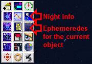
 • NIGHT INFO: It is a list that, for the current night, shows twilights,
sun, moon and some low-accuracy planetary ephemeredes, together with horizontal
data for the main stars. Activate it with the icon showing the moon on the sea
(Main/Viewer tab).
• NIGHT INFO: It is a list that, for the current night, shows twilights,
sun, moon and some low-accuracy planetary ephemeredes, together with horizontal
data for the main stars. Activate it with the icon showing the moon on the sea
(Main/Viewer tab).
• EPHEMEREDES FOR THE CURRENT OBJECT: It shows the
azimuth and height evolution for the current object, the Sun and the Moon.
For periodical variable stars, the instants of
maximum or minimum are also given. The most important data (height vs. time) can
also be seen graphically in the Info tab (see below).
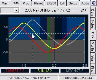
• SPECIAL INFO PLOTS: In addition, some special plots are
displayed to make planning the observation easier:
|
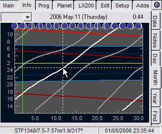
(a) Daily plot (Info/Day tab)
It shows the height trails vs. time for the Sun, Moon
and current object. Daylight conditions (light blue), twilights (dark blue)
and moonlight conditions (grey) are also plotted. The actual night window
(without Moon and in astronomical conditions) appears plotted as dark area.
Use the mouse to read the data (the last line gives the
values for the Sun, Moon and target object). The combo box in the upper left
corner allows changing the current object (target) by any of the main
planets.
|
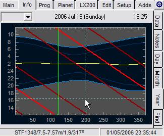
(b) Month plot (Info/Month tab)
A plot showing the instants of upper meridian transit,
rise and set for the current object (deep red = rise and set / bright red=transit),
and the Moon (grey=rise and set / white = meridian). The night time is
represented by the inner black area. Astronomical twilights are the blue
lines, and the grey outer areas represent Sunlight time. As above, the combo
box in the upper left corner allows changing the current object (target) by
any of the main planets. Moon phase is indicated in the top line. The
midnight instants are represented by the central yellow line.
|
|
|
|
|
(c) Annual plot (Info/Year tab)
This plot allows to visualise the instants of rise,
transit and set for the current object (or the planets, using the upper combo
box), together with twilights. The midnight instants are represented by the
central yellow line.
|
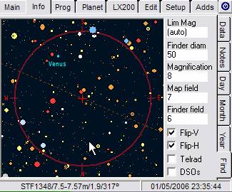
(d) Finder plot (Info/Find tab)
It simulates the finder area, by specifying the
naked-eye weakest star, finder diameter and magnification, and true field.
The finder limiting magnitude is by default auto−calculated.
|
|
|
|
• CALCULATION OF VISIBILITY: It works equally well
for stellar and nonstellar objects. Calculation of
visibility includes locating the optimal combination of eyepieces, Barlow
lenses, and focal reducers.
 The prediction system is explained in
detail in the auxiliary documentation. To learn how it works, activate the Help
pop-up menu, and select the entry "Prediction of visibility". It is
based in the direct use of the Blackwell's response surface giving the eye
detection performance. It is particularly good for small and faint deep sky
objects, but it works even for planets in daylight conditions, or for stars in
night conditions.
The prediction system is explained in
detail in the auxiliary documentation. To learn how it works, activate the Help
pop-up menu, and select the entry "Prediction of visibility". It is
based in the direct use of the Blackwell's response surface giving the eye
detection performance. It is particularly good for small and faint deep sky
objects, but it works even for planets in daylight conditions, or for stars in
night conditions.
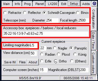
 Activate
it by clicking on the icon with an eye. The telescope and night configuration are specified
in the Setup/Configuration tab. The results are shown in a table arrangement.
Each line corresponds to a combination of eyepiece, barlow lens or focal reducer, from the data you have
indicated in the Setup/Configuration tab, "Accessory box" entry (see
the picture). The telescope diameter and focal length, the naked-eye limiting
magnitude, and the telescope class are used to perform the calculations.
Activate
it by clicking on the icon with an eye. The telescope and night configuration are specified
in the Setup/Configuration tab. The results are shown in a table arrangement.
Each line corresponds to a combination of eyepiece, barlow lens or focal reducer, from the data you have
indicated in the Setup/Configuration tab, "Accessory box" entry (see
the picture). The telescope diameter and focal length, the naked-eye limiting
magnitude, and the telescope class are used to perform the calculations.
The selected line indicates the best eyepiece combination (in
the example, the best combination is a 7 mm with 0.63 focal reducer, which
yields a magnification of x225).
TLM is the telescopic limiting magnitude,
that is, the faintest star seen at the telescope at that magnification
 Most
of the remaining figures are non-intuitive and you have to should read the help
article to understand them. Darkening is the magnitude darkening of the background owing to
the magnification. Backgr is the apparent surface brightness of
the background in magnitudes by squared arc second. SBlim is faintest visible surface
brightness at that magnification in magnitudes by squared arc second. log(C) is the critical contrast. These are
only intermediate calculation results of interest if you have learned the basis
of the prediction of visibility system.
Most
of the remaining figures are non-intuitive and you have to should read the help
article to understand them. Darkening is the magnitude darkening of the background owing to
the magnification. Backgr is the apparent surface brightness of
the background in magnitudes by squared arc second. SBlim is faintest visible surface
brightness at that magnification in magnitudes by squared arc second. log(C) is the critical contrast. These are
only intermediate calculation results of interest if you have learned the basis
of the prediction of visibility system.
Visibility is the final result. If it is larger than zero, the object
can be seen. This value is the only one of importance for most observers in
practice.
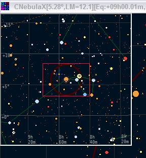
In
this case, with my 254 mm Schmidt-Cassegrain, NGC
6277 is at the eye threshold if we set the appropriate eyepiece combination. For
instance, this galaxy cannot be seen up to reach ca. x100 because the
background is still too luminous for the eye detection capabilities
(visibility<0). The larger the visibility value, the easier the object
with that eyepiece combination. The best eyepiece combination is thus a 7 mm
eyepiece with x0.63 focal reducer-field flattener. If we increase the
magnification too much, it becomes too faint to be perceptible. In this case,
if the magnification exceeds x500, it is lost again because the eye cannot
glimpse a so weakened object.
If
the calculations exceed the response surface area, the line is labelled as
"[extrap]" indicating that the results
should be taken with caution since they come from an extrapolation. NGC 6277 is
anyway a hard object under moderately good rural sky (naked-eye limiting
magnitude 6.5), since the visibility value is quite close to zero.
Just
below the list of magnifications, you will see a line telling whether the
object can be seen, cannot be seen, or it is at the threshold. Three more lines
follow showing the minimal, optimal and maximal magnification at which the
object can be seen. Also, the limiting magnitude that can be detected at those
magnifications, for both a stellar object and a non-stellar object having the
same size that the current one. The last line gives the maximal stellar
magnitude and the minimal magnification required to reach a background of 27
magnitudes by squared arc second. This is the magnification that allows
reaching the maximal stellar magnitude for your instrument and night
conditions.
To top

• MAIN MAP CAPTION: It constantly displays information
about the position pointed by mouse in the main map, together with the map
parameters. You can modify the displayed data from the Main/Map tab. By
default, it can be read the following information:
(1) Current zoom (vertical magnification) in the main map
(2) Limiting magnitude (weakest plotted star)
(3) Equatorial coordinates 2000.0 (RA and DEC)
(4) Constellation code
(5) Chart for Uranometria 2000
(first and second edition: u1 and u2)
(6) Chart for Sky Atlas 2000 (s)
(7) Chart for the Millennium atlas (chart and volume,m)
(8) Chart for Herald-Bobroff chart
(section C, HBc).
(9) Horizontal coordinates (azimuth and height over the
horizon)
(10) Instants of rise,
transit through the upper meridian, and set
 • MEASURING DISTANCES AND POSITION ANGLES ON THE MAIN MAP:
Left click pressing ALT while you drag
the mouse. Release the mouse button and then the ALT key to return to the
normal mode.
 • THE NAVIGATOR: For knowing the Sky area where we are (high zooms), to make
working at a high magnification easier, there is a special second wide view,
called the "navigator" (left upper corner of the main map). You can
use it to zoom or quickly change the position in the main map. The navigator
allows knowing where we are on a large zoom, and it is useful to jump or change
the magnification easily without loosing a high power view of the main map.
• THE NAVIGATOR: For knowing the Sky area where we are (high zooms), to make
working at a high magnification easier, there is a special second wide view,
called the "navigator" (left upper corner of the main map). You can
use it to zoom or quickly change the position in the main map. The navigator
allows knowing where we are on a large zoom, and it is useful to jump or change
the magnification easily without loosing a high power view of the main map.
The Navigator is by default disabled. There are two ways to activate the
navigator:
(1) Click navigator option
button in the Main/Config tab. Clicking
on the "Navigator" icon shows the navigator, and clicking again will
hide it.
(2) Click the navigator icon in the
Main/Viewer tab. Clicking again hides it.
 • THE FINDER VIEW: It is similar to the Navigator. The viewer includes a
special mode (select it from the viewer mode combo box), called
"finder". In "finder mode", the viewer shows a wide map
whose scale can be changed with the slider at the right. Clicking on the finder map, the main map is centred in
the clicked area and the finder, update to that center.
However, magnification changes are only available from the navigator or from
the main map.
• THE FINDER VIEW: It is similar to the Navigator. The viewer includes a
special mode (select it from the viewer mode combo box), called
"finder". In "finder mode", the viewer shows a wide map
whose scale can be changed with the slider at the right. Clicking on the finder map, the main map is centred in
the clicked area and the finder, update to that center.
However, magnification changes are only available from the navigator or from
the main map.

• DSO OBJECTS IN THE FIELD: The data of all plotted objects in
the main window can be listed by clicking on the "DSO in the field"
button .Clicking repeatedly on the button toggle this region on and off. When
it is activated, a list is displayed at the top of the map will the data of all
plotted objects:
(1) Click on the
list to jump to any object displayed on the map.
(2) Click on any
object in the map and get the full information in the upper list.
To top
 • BASIC DATA: NebulaX includes an elaborate way to
prepare observation lists (or programs) that we will see later. However, there
is also a fast procedure: Each time you right click with the mouse on an
object its
basic data are copied to the clipboard (just paste it in MS Word and you will
get a handy observation program), so you can quickly made an observation
program just clicking on the object icons, checking the data, and if you want
to store it in your observation program, pasting its data in your text editor.
You will get for instance this information set in the clipboard when you right
click on M 75:
• BASIC DATA: NebulaX includes an elaborate way to
prepare observation lists (or programs) that we will see later. However, there
is also a fast procedure: Each time you right click with the mouse on an
object its
basic data are copied to the clipboard (just paste it in MS Word and you will
get a handy observation program), so you can quickly made an observation
program just clicking on the object icons, checking the data, and if you want
to store it in your observation program, pasting its data in your text editor.
You will get for instance this information set in the clipboard when you right
click on M 75:
NGC6864/M75 20 06.1 -21 55 SGR GLOCL:1/8.6m/6.0'
343u1/144u2/23s/1386-3m/60HBc
The predictions of visibility and
ephemeredes can be saved on disk as well. The clipboard is available to
transfer more kind of data.
• IMAGES AND
MAPS: From the either Edit tab, from the pop-up menus, or from the Main/Viewer
tab a wide variety of maps (from 250-400 to 4000 pixels) can be copied to be
pasted further in any other application. Also, pictures can be copied and
pasted.
• PASTING DATA: The RTF editor can
be used to place your notes at the telescope, but also accept pictures, maps
and other data. You can make sketches with Paint or scan them, and paste the
images within your own notes.
• PRINTING
MAPS: High resolution maps can also be printed from the Edit tab through the windows default
printer. A certain degree of customisation can be set:
(1) Set the line width from the upper left combo
box.
For laser printers, the lines should be preferably wider (3 points are usually
good).
(2) Modify the star limiting magnitude from the upper
slider labelled with "Mag"
(3) Increase/decrease the star size from the "Star Size" slider.
Usually, 2.5 is quite good for laser printers.
(4) Increase the default deep sky objects from the
"Details" slider
You
can choose printing monochrome maps (black objects on a white background),
colour objects on a white background, or fully customised colours (those
specified in the Setup/Custom colours tab). There is a preview facility in the
Edit tab (star size is not representative in the preview since the printed area
is larger: stars will appear smaller in the printed map).
To top
One of the most important features of CNebulaX is making observation lists. Observation lists
allows jumping to any included object and plotting marks in the main map, and
can be saved for further usage and introduced in word-processing programs. Save
and load lists at your will. Observation lists can be generated mainly in two
ways that can be used in a cooperative fashion:
 • THE PIN ICON: During map exploration, when you find
an object you are interested in, first right click on it to make the active
object. Then click on the Pin icon (the first icon from the left in the
Main/Viewer tab). This will include the object in the observation list, and you
will see a circle highlighting it in the map to visualise it. Adds to the
observation program can also be done from the main map pop-up menu.
• THE PIN ICON: During map exploration, when you find
an object you are interested in, first right click on it to make the active
object. Then click on the Pin icon (the first icon from the left in the
Main/Viewer tab). This will include the object in the observation list, and you
will see a circle highlighting it in the map to visualise it. Adds to the
observation program can also be done from the main map pop-up menu.
 • THE
PROG TAB: The most practical way of making
lists is from the Prog tab, which includes three
secondary tabs that should be used in the following order:
• THE
PROG TAB: The most practical way of making
lists is from the Prog tab, which includes three
secondary tabs that should be used in the following order:
• Database selection: select the
database(s) to be used. The default database is "General", a wide−purpose mixed database good for most situations.
Don't introduce excessive databases or you will slowdown the program
excessively.
• Cross-search: define the
conditions to govern the search. If you want to clean all the text entries, press
the [Clean] button. Empty fields will not condition the search (i.e., they are not
used in the search). A typical search could be for instance finding all
planetary nebulae in Sagittarius brighter than 12.5 magnitude
and larger than 15 arcseconds above -30º declination.
When you have set the search conditions, press [Proceed] to make the search. Remember
to clean the observation program before proceeding to a new search. If you do
not clean it, the new search will be added to the old list. This is indeed a
second possibility: make cumulative searches, provided you make a new search
keeping the old list without cleaning it. You can remove the duplicated objects
using the verify button in the Manage Output tab.
• Manage output: see and edit the
results found, that can be saved on disk, adjoined, or used to explore. Double
click on the list to jump to the objects. Click on the name and wait for a
while to see the data for the clicked object. The final list can be saved in
ASCII format for further use, and cumulative searches are possible to build a
composite list.
 By
default, all the objects that in a given moment are included in the observation
list (Prog/Manage Output tab), are plotted in the
main map as full circles overlaid without labels. Zooming to >100º includes
also additional labels. The markers can be hidden un-checking [Plot list] in the mentioned tab. At
higher magnifications, if a given object is too faint to be auto displayed,
only the circle will indicate that there is an object in the program in that
point. In such situations, if you want to write labels for marking all objects,
check the box [Force labels]. Also, you can change the colour of the labels and the circles from the
same tab.
By
default, all the objects that in a given moment are included in the observation
list (Prog/Manage Output tab), are plotted in the
main map as full circles overlaid without labels. Zooming to >100º includes
also additional labels. The markers can be hidden un-checking [Plot list] in the mentioned tab. At
higher magnifications, if a given object is too faint to be auto displayed,
only the circle will indicate that there is an object in the program in that
point. In such situations, if you want to write labels for marking all objects,
check the box [Force labels]. Also, you can change the colour of the labels and the circles from the
same tab.
That [Manage Output] tab allows some
additional facilities:
Clear: It empties the list and removes all
the markers in the main map
Load: Load a previously saved observation
program. It can be used in a cumulative way, appending to the current list an
older one. After the loading, some objects can be repeated: use the verify button to remove
repetitions and sort the merged list.
Save: Save the current observation program
in the hard drive for further usage.
Del Marked: Remove particular entries in the upper list (those
one that are marked). To mark several objects and remove them in a single
operation, combine mouse left clicks with the keys SHIFT and CTRL, as in any
windows application.
Show: Display the list in a more complete fashion.
Click on the new list to jump to the objects. This list can also be displayed
from an icon in the Main/Viewer tab.
Inverse: Inverse the selection state (unmark
marked lines and vice-versa)
Verify: Remove repetitions and sort the list
Besides
these procedures, remind that each time you right click on any object plotted
in the main map, its basic data are transferred to the clipboard: paste them in
a word processing program, or in any window that accept them (the CNebulaX quick notebook, the user notes, etc)
For
a quick activation, there is an icon in the Main/Viewer tab that directly
displays the full list.
To top
There are two ways
of taking notes:
 • QUICK NOTES: CNebulaX includes an area to write down
notes of any kind. These quick notes are auto-saved in a text file called Notebook.txt (RootCNebulaXFolder).
This file is loaded each time the program is started, so it is a matter of
diary. I use the quick notes area to store annotations about the objects I want
to observe because present special interest. Normally, once found an object I
am interested in, I paste the basic line in the notebook area and I add the
comments that moved me to select the object. But naturally, you can write in
the notebook any piece of information.
• QUICK NOTES: CNebulaX includes an area to write down
notes of any kind. These quick notes are auto-saved in a text file called Notebook.txt (RootCNebulaXFolder).
This file is loaded each time the program is started, so it is a matter of
diary. I use the quick notes area to store annotations about the objects I want
to observe because present special interest. Normally, once found an object I
am interested in, I paste the basic line in the notebook area and I add the
comments that moved me to select the object. But naturally, you can write in
the notebook any piece of information.
When you want to return to the map, press
either the ESC key or the close button of the main map. The notebook file is
auto-saved when you return to the main map, if the program detects changes.
• TAKING NOTES
AT THE TELESCOPE: Notes relative to the active object including pictures,
maps or photos can be introduced using the Info/Notes tab. The notes are saved
in individual files stored in the "notes" folder. If the program
detects changes, it will display the save dialog, but you can save the notes at
any time pressing the "save" icon.
 Advising
if the current object includes notes - The notebook icon (quick notes,
Main/Viewer tab) changes to indicate whether the active object includes notes
or not. When the current object includes additional notes, the icon background
becomes green whereas the notebook colour changes form white to yellow.
Advising
if the current object includes notes - The notebook icon (quick notes,
Main/Viewer tab) changes to indicate whether the active object includes notes
or not. When the current object includes additional notes, the icon background
becomes green whereas the notebook colour changes form white to yellow.
To top
The release 1.05 includes finally calculation
of orbits for comets and minor planets. In addition, it is also prepared for
applying the VSOP87 theory (the main planets). Pluto
is still not available.
 Go to the Planet/Comet tab. Then specify the search
limit in astronomical units (by default, it is 4 AU, beyond which the comets
are usually too faint). Finally, push the Load button to search the comets in the database,
and load them. If you want to restrict the search, write in the "name
pattern" box the name mask to be applied. For instance, if you write
"Bro", the comets to be loaded will be "Brorsen",
"Pons-Brooks", "Brooks
2", etc. You likely need to extend the AU search limit to load a very
distant comet.
Go to the Planet/Comet tab. Then specify the search
limit in astronomical units (by default, it is 4 AU, beyond which the comets
are usually too faint). Finally, push the Load button to search the comets in the database,
and load them. If you want to restrict the search, write in the "name
pattern" box the name mask to be applied. For instance, if you write
"Bro", the comets to be loaded will be "Brorsen",
"Pons-Brooks", "Brooks
2", etc. You likely need to extend the AU search limit to load a very
distant comet.
The search text box - You can search the comets in
the list: write the search pattern (i.e., "Poj" for
Pojmanski), in the search text box, and press ENTER
repeatedly up to jump the Pojmanski comet. In this case, there
is only one comet matching the search conditions, so you will get it
immediately. Once the comet is selected, it is available for centring the map
on it (jump button), or for loading the orbital elements to calculate
ephemeredes and orbital trails (trace button).
The Trace button - When you have loaded the currently
visible comets filling the list below (for each comet, it lists constellation,
magnitude, number and name), they will plotted in the main
map and are available to jump to them (select one comet and press the
"Jump" button). However, if you want more ephemeredes for a
particular comet, then click on the "Trace" button. This will load
the orbital elements and activate the Planet/Trace tab, which allows checking
how the magnitude, phase angle, elongation, and distances to the Sun and to the
Earth changes with the time (combo box above).
Orbital trails - The trace button also allows tracing
the orbit for comets, asteroids and planets covering different periods (1 year,
6 months, 3 months, etc; combo box below). Select the time period and jump to
the object to see the trail. For removing the trail selecting
"(none)" in the combo box.
Overlay external tables - In addition to the
CNebulaX orbital trails, you can also represent
external ephemeredes from the Adds/Overlay tab. Make an ASCII file containing
only columns of data, and add a first line with the following decoding
characters:
Identifier: L=labels [Pojmanski]= LLLLLLLLL
Right Ascension: H=hours,
M=minutes, S=seconds [11h12.34m]= HH MMMMM
[11
12 34.3]= HH
MM SSSS
[11.245]=
HHHHHH
Declination: +=sign, º=degrees,
'=minutes, "=arcsec [11º12.34']= ºº '''''
[11
12 34.3]= HH
'' """"
[11.245]=
ºººººº
An example with the first 5 rows of a
hypothetical file containing a table of ephemeredes, with the corresponding
decoding header in the first line could be:
 Comets at scale - Comets are plotted at scale,
orienting the tail opposite to the Sun and with a standard length and size
(merely informative) of 10 million kilometres. The comma is also indicative of
the comet scale, and by default it is 1 million kilometres width. These figures
correspond to perihelium values, and give an
indication on how far the comet is and its real orientation in the sky.
Comets at scale - Comets are plotted at scale,
orienting the tail opposite to the Sun and with a standard length and size
(merely informative) of 10 million kilometres. The comma is also indicative of
the comet scale, and by default it is 1 million kilometres width. These figures
correspond to perihelium values, and give an
indication on how far the comet is and its real orientation in the sky.
The magnitude of comets is rather uncertain.
The default values (Planet/Model tab) allow having an approximate idea of a
usual comet, but bright comets are exceptional and can differ strongly. The JPL
database used here with ca. 2,500 comets does not include absolute magnitude
and slope, and the magnitude previsions are done with the default values, so
they must be taken with caution.
Deep searches - The loading capacity is restricted to
2500 asteroids and 300 comets (far more than enough) in the whole sky. However,
you can load a very deep search restricting the search to the current map
(marking the respective check box). In this way, you can for instance load
asteroids up to 24th magnitude or any known comet, and get an extremely deep
chart for the region you want.
It has the same structure and similar features
than the facilities for comet predictions introduced just above (read it). In
this case, however, magnitudes are well known and predictions are reliable. So
the search limit is done in this case attending to the visual magnitude. There
are ca. 300,000 asteroids, in three databases provided by the Jet Propulsion
Laboratory (JPL):
(1) Brief database (default) - Asteroid with a common
name (ca. 12,000)
(2) Full database #1 - Secure (numbered)
asteroids, with accurate data (ca. 100,000)
(3) Brief database #2 - Asteroids with
inaccurate orbital elements or few observed (ca. 200,000)
The brief database covers by far all the needs
of amateurs and it is fast to load, so use it except for power searches. The
default magnitude parameters can be specified in the Planet/Model tab.
You can specify a name pattern if you want to
restrict the search to a few, or a singe asteroid. Also, you can restrict the
loading to the asteroids appearing in the current chart. The result list will
show the asteroids sorted by constellations and visual magnitude.
By default, CNebulaX
uses a low accuracy theory to predict planets (based on the VSOP82
theory), except when the area is magnified (zoom<25º). However, more
accurate predictions are available from the Planet/Planet tab. The Trace button here give access to evolution plots in the same way
as for comets and asteroids. Also, the planets trails can be plotted form the
trace tab. Read the information given above for comets to know the details.
From the 1.05.65 rs,
main planets, asteroids, and comets, are given in topocentric
apparent equatorial coordinates, with an accuracy
higher than 0.05 arc seconds with regard to USNO
ephemeredes. The Moon remains uncorrected, and Pluto is still not implemented (1.05.65rs).
To top
This is one of my favourite features (activate
it from the book icon with an R in the cover). It includes navigating tables
(click on an object row to center that object in the
map) through combo boxes. The main use is listing what any constellation
contains. But the first combo (on the left) gives access to other very handy
sections, including references and thousands of observations found in the
internet, lists by DSO type, astrophysical data and so on. Take your time
exploring this, IT IS REALLY HUGE.
Compiling files in the help format
is not included in this release yet. If you have a file with information you
think could be of interest for other people and would like to include in the
reference library, send me the file and I will compile it for the inclusion.
The use of the library is simple. There are
three combo boxes in the top line. The left one is the main combo: deploy it to
list the main items. The central combo is the secondary combo and includes the
subtopics related to the each main combo entry. Identically, the third combo at
the right includes the subtopics associated to each second combo item. Just
click on them to deploy the information. There are quite tables listing brief
data: clicking on them will move the main map to the listed objects. To refresh
the screen, change the main combo item to another one.
Each time you leave the reference library, the
position within the list is kept. Thus, just click again the Ref icon and you
will be ready to follow with the data in the same place where you were.

The command controls in the second line are:
• Autocons: if it is checked,
the constellation list is changed to follow the active object in the Main Map
• Get Constel: pressing the button changes once the list to the
constellation of the active object
• Search
facility: type in the textbox the string to be searched in the list below. Then
press the find button repeatedly up to get the line you want to locate.
Finally, press the jump button to center the map in the
object found.
• Bookmarks: The remaining
buttons in the second row set up to three bookmarks in the help system. Once
set a marker (set button), clicking in the respective go button will move the
help system to the stored bookmark.
To top
 CNebulaX was originally designed to assist my 10"
Meade LX200 classic, and it includes controls to govern it. I have had no
opportunities to try other telescopes, but I am considering implement the ASCOM standard in the near future. At the moment, the
current LX200 control can be used in other telescopes with emulating
interfaces.
CNebulaX was originally designed to assist my 10"
Meade LX200 classic, and it includes controls to govern it. I have had no
opportunities to try other telescopes, but I am considering implement the ASCOM standard in the near future. At the moment, the
current LX200 control can be used in other telescopes with emulating
interfaces.
The interface is transparent: the orders sent to
or received from the serial port can be seen in a monitor (LX200/Port monitor
tab). There are two ways of slewing the telescope to point an object. First you
should configure the RS232C (LX200/Serial port setup), and open the connection
(LX200/Telescope tab). Then, you can govern it very easily from the Main/Viewer
tab, or from the LX200/Telescope tab:
(1) By
clicking the icon with a telescope in the Main/Viewer tab. For doing this,
first right click on the object in order to make it the active object.
Then press the small icon with the telescope icon to slew to it (Main/Viewer
tab).
In the LX200/Telescope tab you will
find another command button for activate slews.
(2) By
clicking a special icon with a gear wheel (a button that as in (1) is placed in
the last row of the Main/Viewer tab). For doing this, first click on that
toolbox icon: you will see that a gear will appear in the middle of the main
map. Now click on this new gear icon holding the mouse, and drag it to
the place where you want to point the telescope, releasing the mouse. You can
repeat the click+hold movement up to situate it exactly
where you want. Finally, click again in the toolbox icon, and the telescope
will move to point the target place.

Similarly, the LX200/Telescope tab
have a similar facility (a check box, in this case). When you mark it,
the gear wheel to be dragged is shown in the screen centre. Drag it to the
target point and press slew telescope (command button above he check box)
(3) Some basic
movement arrows can be used from the Main/Viewer tab. This is hidden
and should be activated by clicking on the left icon in the same row as (1) and
(2), in the Main/Viewer tab.
Additional controls are available in the LX200 main tab: information
about position and time sent from the LX200, and synchronisation between
telescope and computer.
To top
This facility is available from the Adds/Image
tab. The fitting requires installing the GSC
databases (if you have not installed it yet, grab it from the website).
 (1) Images should be
first resized with an external program if they are larger than the screen when
zoomed at 100%, with photoshop, irfanview
or whatever similar program. The best performance is when the image fills
completely the screen at 100%. At the moment, CNebulaX
does not resize them, but it will in next revisions. The program can process rotated
images, but should be un-inverted. Flipped images cannot be processed, and should be
flipped manually from an external program.
(1) Images should be
first resized with an external program if they are larger than the screen when
zoomed at 100%, with photoshop, irfanview
or whatever similar program. The best performance is when the image fills
completely the screen at 100%. At the moment, CNebulaX
does not resize them, but it will in next revisions. The program can process rotated
images, but should be un-inverted. Flipped images cannot be processed, and should be
flipped manually from an external program.
(2) Go to the Adds/Image
tab. Load the picture with the folder button. The picture will be set at the
background. Note that the usual appearance of the map will be different: the program will
enter in the so-called "markers mode", which allows
fitting images and maps. In the markers mode, mouse clicks will place
markers on the map instead of re-centring the image. Markers are reference
points to match the image with the map.
(3) You should
establish the equivalence between map and picture by setting two pairs of
reference points, common to the map and the photo. These 4 points are [Atlas-1]
to match with [Photo-1]), and [Atlas-2] to match with [Photo-2].
To establish the equivalences, you can use whatever feature you could identify
in the picture that is also plotted in the map: stars, the cores of deep sky
objects, a prominent knotty nebula, etc. And you can make corrections by
iterations (make a guess and try). The four markers needed are selected with
the four option buttons you will see in the toolbox.
(4) Then press
[rotate + scale] button to change scale and orientation. This will rotate and
change the magnification of the map, and will return to the normal mode.
The centres, however, are not coincident.
(5) After
re-scaling, CNebulaX will return to the normal mode
("markers" check box unelected). Click repeatedly near the central
cross to move the map gradually to match the picture. For small corrections,
you can also use:
·
The two rotate
buttons for slight rotations
·
The four move
buttons for slight movements in the final adjustments
The center can also be adjusted with one or two pairs of reference
points with the [Move] button. However, final adjustments are always needed.
(6) If you discover
that you had to do a major correction, or need to re-scale, check again the
"Markers" checkbox and repeat the process from step (3).
(7) When all is at
your taste, click the "save" button to save the final image:
·
For saving conventional
stars,
uncheck the "Markers" checkbox
·
For saving no stars, uncheck the
"Stars" checkbox
·
For saving the
stars as empty circles check the "Circles" checkbox
·
For saving semi-transparent
stars (recommended),
check "Markers" and choose the colour you wish (colour diagram
button)
To top
