Next: 2.6 Magnetohidrodinámica Ideal Up: 2.5 Relativistic Hydrodynamics Previous: 2.5.1 Equations of Relativistic
Let us introduce into system (122) the Jacobian matrices
![]() associated to the five-vectors
associated to the five-vectors
![]()
Finally, we introduce the vectors
| (57) |
With the above definitions, system (122) reads as a system of
conservation laws
for the new vector of unknowns u
In the above system (59) we can define three
![]() -Jacobian matrices
-Jacobian matrices
![]() (u),
the Jacobian matrices associated to the vector
(u),
the Jacobian matrices associated to the vector
![]() (u), the flux in the
(u), the flux in the ![]() -direction
of the system (59), as:
-direction
of the system (59), as:
Following a procedure similar to the one described in
Font et al.(1994) we have succeeded in obtaining analytical expressions
for the spectral decomposition of the matrices
![]() (u).
For the sake of clarity, let us restrict to a 2D case, i.e., to problems
involving a dependence on two spatial coordinates (that we will denote
with the scripts i = x, y instead of i = 1,2)
(u).
For the sake of clarity, let us restrict to a 2D case, i.e., to problems
involving a dependence on two spatial coordinates (that we will denote
with the scripts i = x, y instead of i = 1,2)
The eigenvalues and the right and left eigenvectors of
![]() (similar for i=y) are going to be displayed explicitly.
(similar for i=y) are going to be displayed explicitly.
The eigenvalues of matrix ![]() (u) are:
(u) are:
Let us make several comments to the above expressions for the eigenvalues:
i) In the case (![]() ),
expression (61) gives the corresponding one-dimensional
eigenvalues
),
expression (61) gives the corresponding one-dimensional
eigenvalues
| (62) |
ii) In the limit
![]() , the genuinely nonlinear
characteristic fields
, the genuinely nonlinear
characteristic fields ![]() become linearly degenerate.
become linearly degenerate.
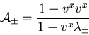
For the sake of concisness and before showing the
complete set of right and left-eigenvectors, let us define
the following quantities:
 |
(63) |
 |
(64) |
| (65) |
A complete set of right-eigenvectors is,
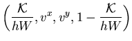 |
(66) |
| (67) |
| (68) |
The corresponding complete set of left-eigenvectors is
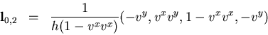
![\begin{displaymath}
{\bf l}_{\mp} = ({\pm} 1){\displaystyle{\frac{h}{\Delta}}}
...
...
{\cal K} {\cal A}_{\pm} {\lambda}_{\pm}
\end{array} \right]
\end{displaymath}](img376.png)
Symmetry relations allow to extend the above spectral decomposition to
the other spatial direction ![]() and also to the general 3D case.
and also to the general 3D case.
As we have emphasized above,
in order to apply HRSC methods to solve the equations of relativistic
hydrodynamics as written in (59), the knowledge of the spectral
decomposition of the Jacobian matrices ![]() is crucial.
is crucial.
![\begin{displaymath}
\lambda_{\pm} = \frac{1}{1- v^2 c_s^2}
\left\{v^{x}(1-c_{s}^...
...{(1-{\rm v}^{2}) [1-v^x v^x-
(v^2-v^x v^x)c_{s}^{2}]}
\right\}
\end{displaymath}](img357.png)