Next: 4.1.2 Exact solution of Up: 4.1 High-resolution shock-capturing schemes Previous: 4.1 High-resolution shock-capturing schemes
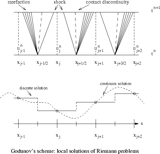
The incorporation of the exact solution of Riemann problems to compute the numerical fluxes is due to Godunov (1959)
Godunov developed his method to solve the Euler equations of classical gas dynamics in the presence of shock waves
Outline of Godunov's method:
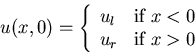
The solution to the Riemann problem at ![]() is a similarity
solution, which is constant along each ray
is a similarity
solution, which is constant along each ray
| (104) |
![]() is the exact solution along the ray
is the exact solution along the ray ![]() with data
with data
 |
(105) |
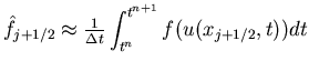
![]() must be small enough so that waves from the Riemann problems
do not travel farther than distance
must be small enough so that waves from the Riemann problems
do not travel farther than distance ![]() in this time step (CFL condition)
in this time step (CFL condition)
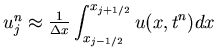
To compute
![]() we must determine the full wave structure
and wave speeds in order to find where it lies in state space
we must determine the full wave structure
and wave speeds in order to find where it lies in state space ![]() computationally expensive procedure
computationally expensive procedure
A wide variety of approximate Riemann solvers have been proposed
![]() much cheaper than the exact solver and equally good results
when used in the Godunov or high-resolution methods
much cheaper than the exact solver and equally good results
when used in the Godunov or high-resolution methods