Next: 4.1.1 Godunov's method Up: 4 Métodos en diferencias Previous: 4 Métodos en diferencias
High-resolution methods: modified high order methods with the appropriate amount of numerical dissipation in the vicinity of a discontinuity
Let us consider the following (Cauchy) IVP
| (97) |
A finite difference scheme
is a time-marching procedure which permits to obtain approximations to the
solution in the mesh points, ![]() , from the approximations in previous
time steps
, from the approximations in previous
time steps ![]()
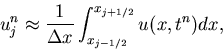
Quantity ![]() is an approximation to
is an approximation to ![]() but, in the case of a conservation law, it is
often preferable to view it as an approximation to the average of
but, in the case of a conservation law, it is
often preferable to view it as an approximation to the average of
![]() within the numerical cell
within the numerical cell
![]() (
(
![]() )
)
 |
(98) |
For hyperbolic systems of conservation laws, schemes written in conservation form guarantee that the convergence (if it exists) is to one of the weak solutions of the original system of equations (Lax-Wendroff theorem 1960).
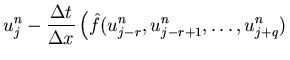
An algorithm written in conservation form reads
| (100) |
The Lax-Wendroff theorem does not state whether the method converges.
To guarantee convergence, some form of stability is required, as for linear problems (Lax equivalence theorem, see Ritchmyer & Morton 1967)
The notion of total-variation stability has proven very successful although powerful results have only been obtained for scalar conservation laws
The total variation of a solution at ![]() ,
TV(
,
TV(![]() ), is defined as
), is defined as
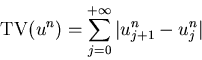 |
(101) |
A convergence theorem for non-linear, scalar, conservation laws (LeVeque 1991): For numerical schemes in conservation form with consistent numerical flux functions, TV-stability is a sufficient condition for convergence
A current line of research focuses on developing high-order, accurate methods in conservation form satisfying the condition of TV-stability
The conservation form is ensured by starting with the integral
version of the partial differential equation in conservation form. Integrating
the PDE within a space-time computational cell
![]() , the
numerical flux function
, the
numerical flux function
![]() is seen to be an approximation to the
time-averaged flux across the interface, i.e.,
is seen to be an approximation to the
time-averaged flux across the interface, i.e.,
| (102) |
The flux integral depends on the solution at
the numerical interfaces,
![]() , during the time step
, during the time step
Key idea:
a possible procedure is to calculate
![]() by
solving Riemann problems at every cell interface to obtain
by
solving Riemann problems at every cell interface to obtain
| (103) |
![]() denotes the Riemann solution for the (left and
right) states
denotes the Riemann solution for the (left and
right) states ![]() ,
, ![]() along the ray
along the ray ![]()