Next: 4.2 Riemann solvers Up: 4.1 High-resolution shock-capturing schemes Previous: 4.1.2 Exact solution of
This is the approach followed by an important subset of shock-capturing methods, the so-called Godunov-type methods (Harten & Lax 1983, Einfeldt 1988)
These methods are written in conservation form and use
Riemann solvers to compute approximations
to
![]()
High-order of accuracy is achieved in two different ways:
A remark: artificial viscosity methods
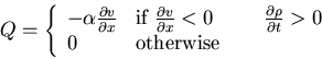 |
(106) |
with
![]()
Flux limiter methods:
The numerical flux is obtained from a high order flux (e.g., the Lax-Wendroff flux) in the smooth regions and from a low order flux (e.g., the flux from some monotone method) near discontinuities
with the limiter ![]()
Example: the flux-corrected-transport algorithm (Boris and Book 1973), one of the earliest high resolution methods
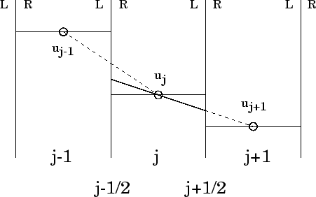
Slope limiter methods:
Use of conservative polynomial functions to interpolate the approximate solutions within the numerical cells
The idea is to produce more accurate left and right states for the Riemann
problems by substituting the mean values ![]() (that give only
first-order accuracy) for better approximations of the true flux near the
interfaces,
(that give only
first-order accuracy) for better approximations of the true flux near the
interfaces,
![]() ,
,
![]()
The interpolation algorithms have to preserve the TV-stability of the scheme and this is usually achieved by using monotonic functions which lead to a decrease in the total variation (total-variation-diminishing schemes, TVD, Harten 1984)
If R is an interpolant function for the approximate solution ![]() and
and
![]() is the interpolated function within the cells, i.e.,
is the interpolated function within the cells, i.e.,
![]() , satisfying
, satisfying
![]() then it can be proven
that the whole scheme verifies
then it can be proven
that the whole scheme verifies
![]() .
.
High-order TVD schemes were first constructed by van Leer (1979) who obtained second-order accuracy by using monotonic piecewise linear slopes for cell reconstruction

The piecewise parabolic method (PPM) of Colella and Woodward (1984) provides third-order accuracy
The TVD property implies TV-stability but can be too restrictive. In fact, TVD methods degenerate to first order accuracy at extreme points (Osher & Chakravarthy 1984)
Other reconstruction alternatives have been developed in which some growth of the total variation is allowed: